mfrmr Visual Diagnostics
Source:vignettes/mfrmr-visual-diagnostics.Rmd
mfrmr-visual-diagnostics.RmdThis vignette is a compact map of the main base-R diagnostics in
mfrmr. It is organized around four practical questions:
- How well do persons, facet levels, and categories target each other?
- Which observations or levels look locally unstable?
- Is the design linked well enough across subsets or forms?
- Where do residual structure and interaction screens point next?
All examples use packaged data and
preset = "publication" so the same code is suitable for
manuscript-oriented graphics.
Minimal setup
library(mfrmr)

toy <- load_mfrmr_data("example_core")

fit <- fit_mfrm(
  toy,
  person = "Person",
  facets = c("Rater", "Criterion"),
  score = "Score",
  method = "JML",
  model = "RSM",
  maxit = 20
)
#> Warning: Optimizer did not fully converge (code = 1). Consider increasing maxit
#> (current: 20) or relaxing reltol (current: 1e-06).

diag <- diagnose_mfrm(fit, residual_pca = "none")
1. Targeting and scale structure
Use the Wright map first when you want one shared logit view of persons, facet levels, and step thresholds.
plot(fit, type = "wright", preset = "publication", show_ci = TRUE)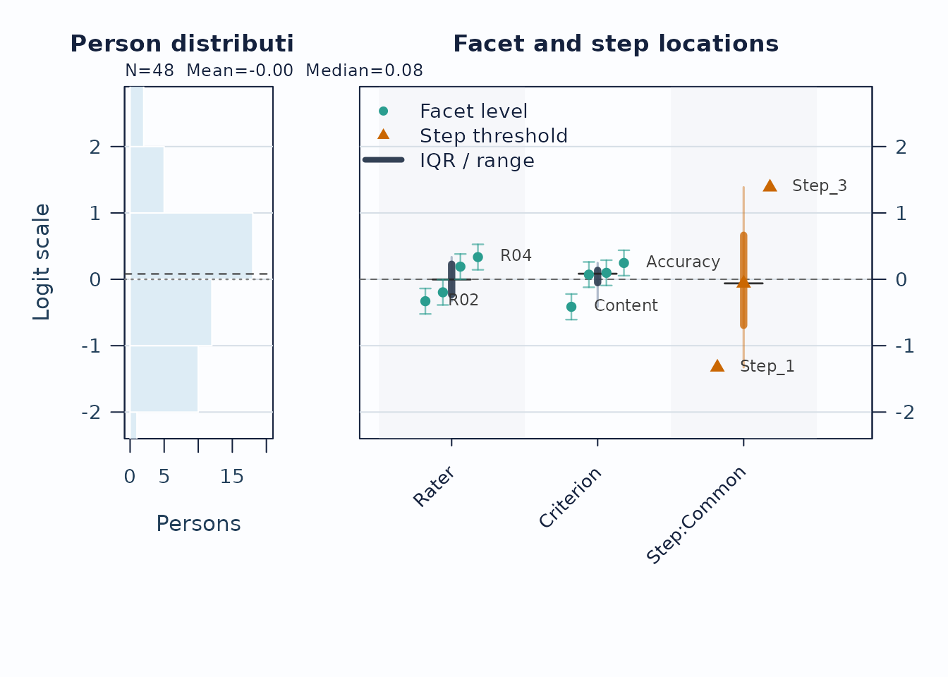
Interpretation:
- Compare person density on the left to facet and step locations on the right.
- Large gaps suggest weaker targeting in that logit region.
- Wide overlap in confidence whiskers means neighboring levels are not cleanly separated.
Next, use the pathway map when you want to see how expected scores progress across theta.
plot(fit, type = "pathway", preset = "publication")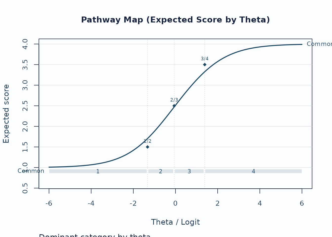
Interpretation:
- Steeper rises indicate stronger score progression.
- Dominant-category strips show where each category is most likely to govern the score.
- Flat or compressed regions suggest weaker category separation.
2. Local response and level issues
Unexpected-response screening is useful for case-level review.
plot_unexpected(
  fit,
  diagnostics = diag,
  abs_z_min = 1.5,
  prob_max = 0.4,
  plot_type = "scatter",
  preset = "publication"
)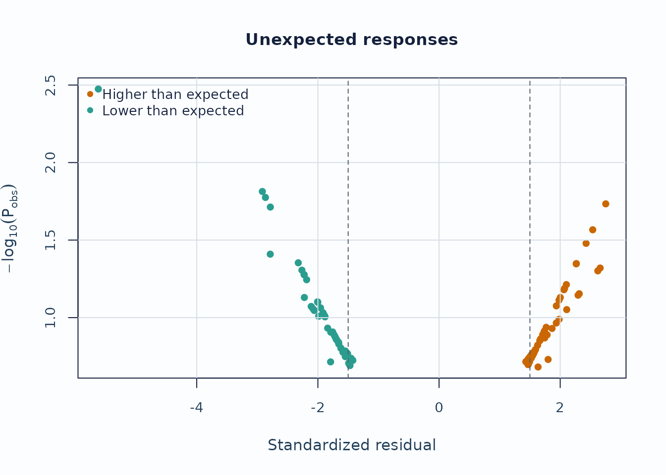
Interpretation:
- Upper corners combine large residual mismatch with low model probability.
- Repeated appearances of the same persons or levels are more informative than a single extreme point.
Displacement focuses on level movement rather than individual responses.
plot_displacement(
  fit,
  diagnostics = diag,
  anchored_only = FALSE,
  plot_type = "lollipop",
  preset = "publication"
)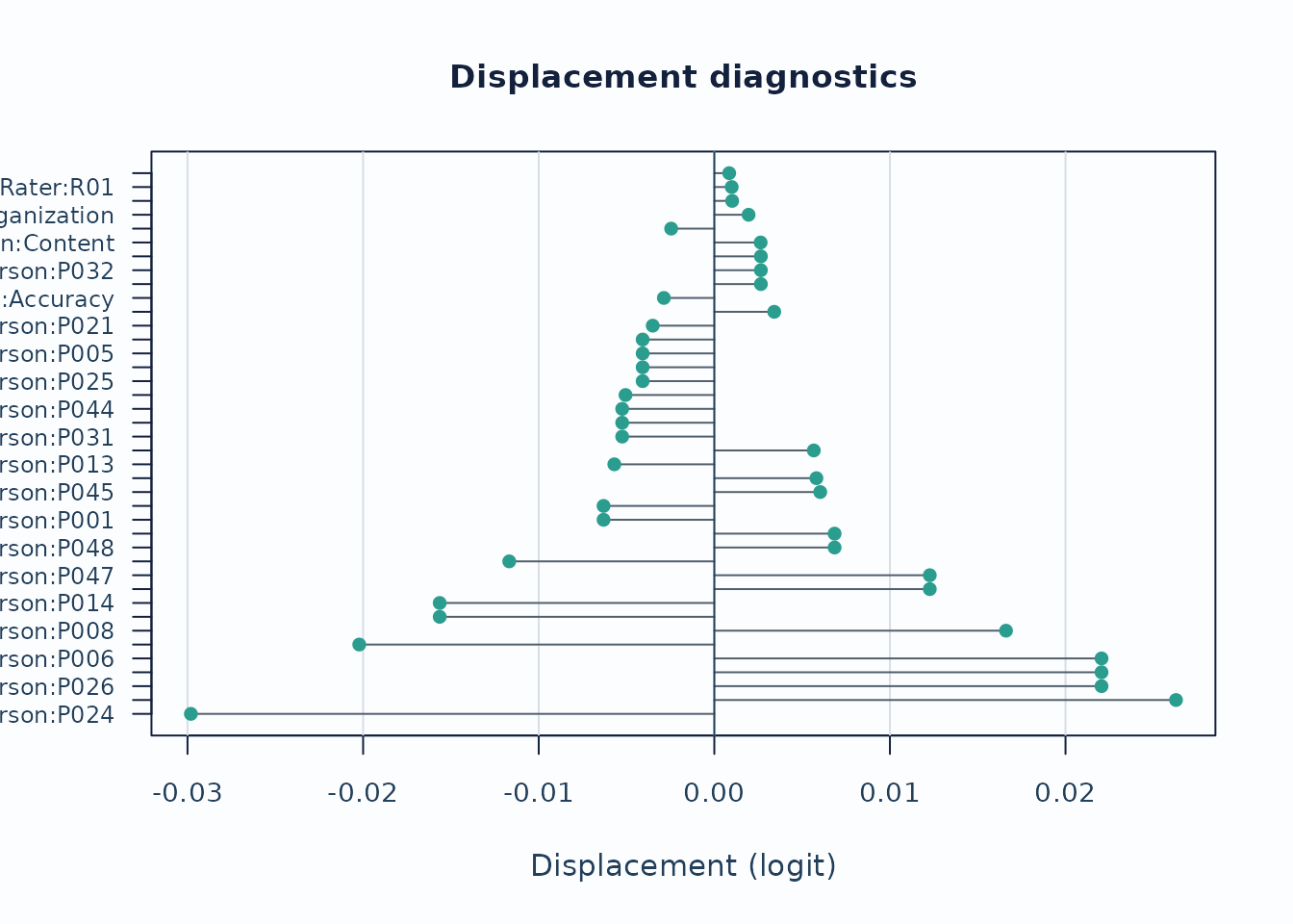
Interpretation:
- Large absolute displacement indicates stronger tension between observed data and current calibration.
- For anchored runs, this is especially useful as an anchor-robustness screen.
3. Linking and coverage
When the design may be incomplete or spread across subsets, inspect the coverage matrix before interpreting cross-subset contrasts.
sc <- subset_connectivity_report(fit, diagnostics = diag)
plot(sc, type = "design_matrix", preset = "publication")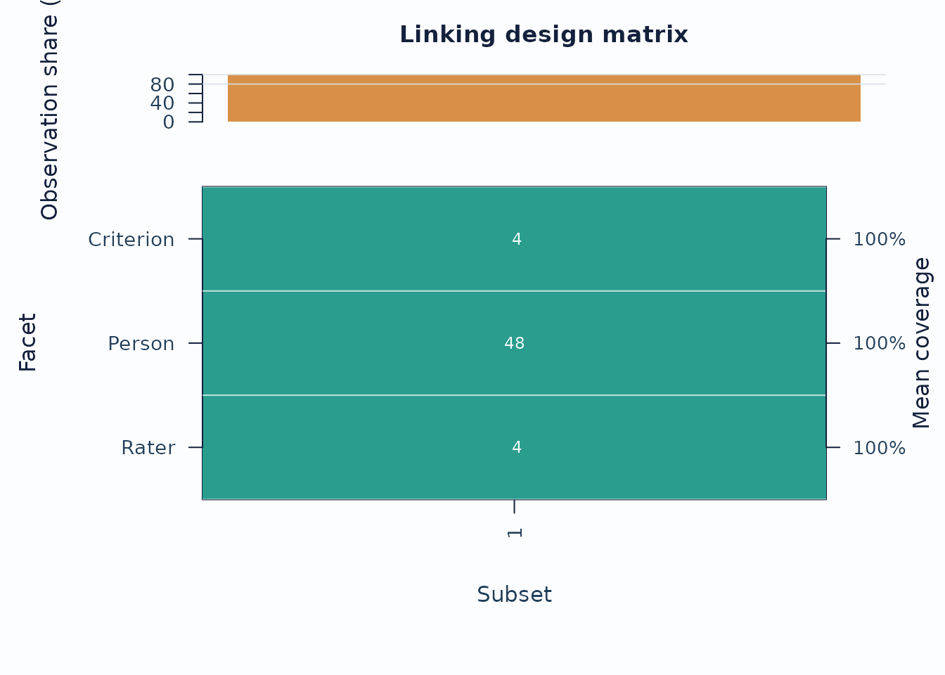
Interpretation:
- Sparse rows or columns indicate weak subset coverage.
- Facets with low overlap are weaker anchors for cross-subset comparisons.
If you are working across administrations, follow up with anchor-drift plots:
drift <- detect_anchor_drift(current_fit, baseline = baseline_anchors)
plot_anchor_drift(drift, type = "heatmap", preset = "publication")
4. Residual structure and interaction screens
Residual PCA is a follow-up layer after the main fit screen.
diag_pca <- diagnose_mfrm(fit, residual_pca = "both", pca_max_factors = 4)
pca <- analyze_residual_pca(diag_pca, mode = "both")
plot_residual_pca(pca, mode = "overall", plot_type = "scree", preset = "publication")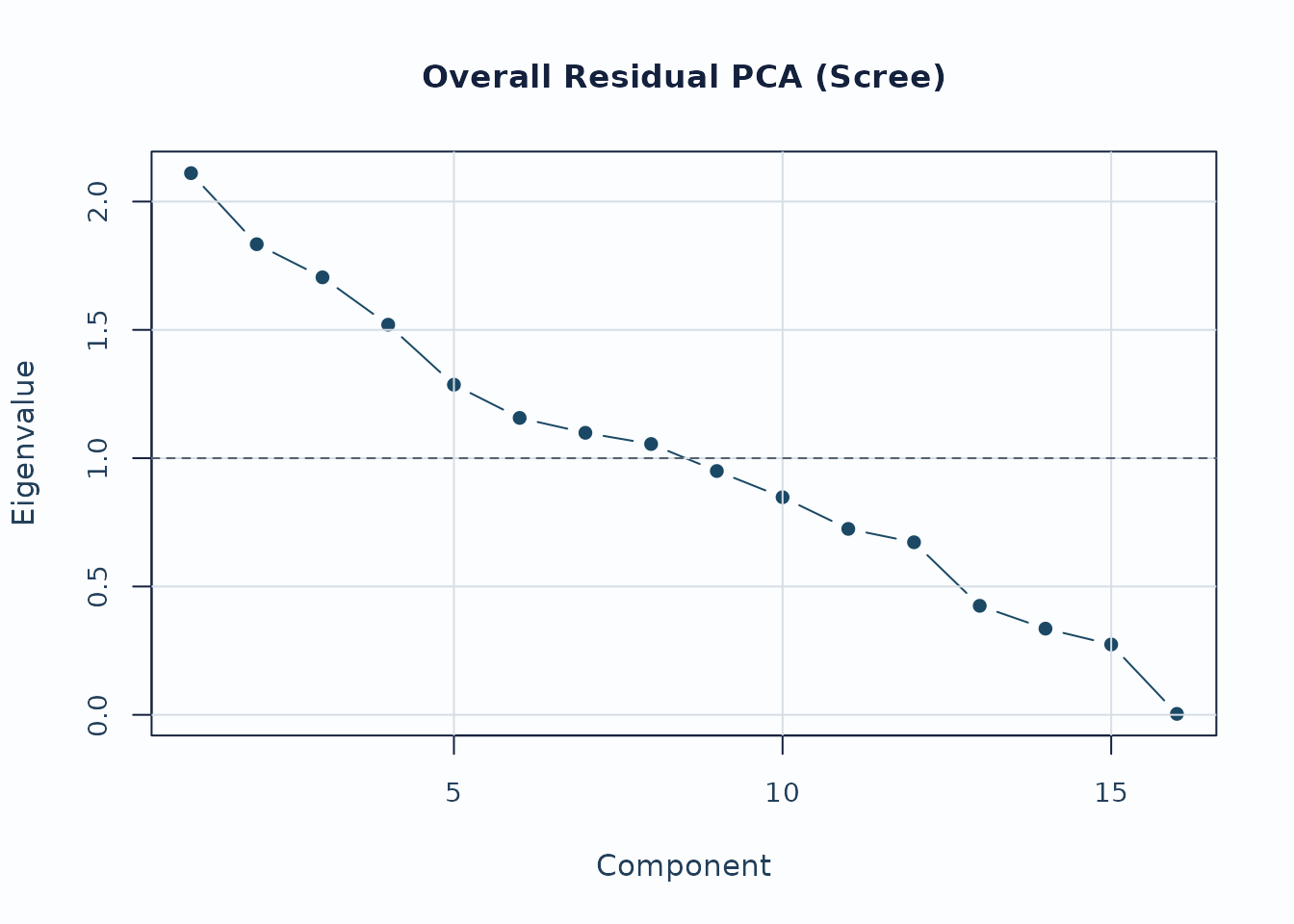
Interpretation:
- Early components with noticeably larger eigenvalues deserve follow-up.
- Scree review should usually be paired with loading review for the component of interest.
For interaction screening, use the packaged bias example.
bias_df <- load_mfrmr_data("example_bias")

fit_bias <- fit_mfrm(
  bias_df,
  person = "Person",
  facets = c("Rater", "Criterion"),
  score = "Score",
  method = "MML",
  model = "RSM",
  quad_points = 7
)

diag_bias <- diagnose_mfrm(fit_bias, residual_pca = "none")
bias <- estimate_bias(fit_bias, diag_bias, facet_a = "Rater", facet_b = "Criterion")

plot_bias_interaction(
  bias,
  plot = "facet_profile",
  preset = "publication"
)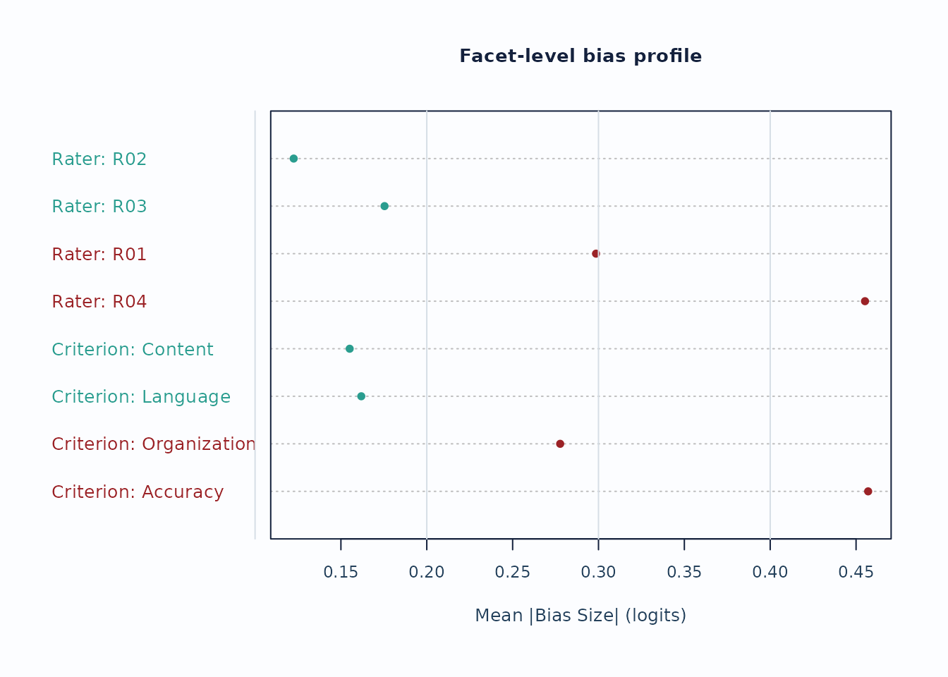
Interpretation:
- Facet profiles are useful for seeing whether a small number of levels drives most flagged interaction cells.
- Treat these plots as screening evidence; confirm with the corresponding tables and narrative reports.
Recommended sequence
For a compact visual workflow:
-
plot_qc_dashboard()for one-page triage. -
plot_unexpected(),plot_displacement(), andplot_interrater_agreement()for local follow-up. -
plot(fit, type = "wright")andplot(fit, type = "pathway")for targeting and scale interpretation. -
plot_residual_pca()andplot_bias_interaction()for deeper structural review.