This vignette outlines a reproducible workflow for:
- loading packaged simulation data
- fitting an MFRM with flexible facets
- running diagnostics and residual PCA
- generating APA and visual summary outputs
- moving from fitted models into design simulation and fixed-calibration prediction
For a plot-first companion guide, see the separate
mfrmr-visual-diagnostics vignette.
For speed-sensitive work, a useful pattern is:
- start with
method = "JML"orquad_points = 7 - use
diagnose_mfrm(..., residual_pca = "none")for the first pass - reuse the same diagnostics object in downstream reports and plots
Load Data
library(mfrmr)

list_mfrmr_data()
#> [1] "example_core"     "example_bias"     "study1"           "study2"
#> [5] "combined"         "study1_itercal"   "study2_itercal"   "combined_itercal"

data("ej2021_study1", package = "mfrmr")
head(ej2021_study1)
#>    Study Person Rater              Criterion Score
#> 1 Study1   P001   R08      Global_Impression     4
#> 2 Study1   P001   R08 Linguistic_Realization     3
#> 3 Study1   P001   R08       Task_Fulfillment     3
#> 4 Study1   P001   R10      Global_Impression     4
#> 5 Study1   P001   R10 Linguistic_Realization     3
#> 6 Study1   P001   R10       Task_Fulfillment     2

study1_alt <- load_mfrmr_data("study1")
identical(names(ej2021_study1), names(study1_alt))
#> [1] TRUE
Minimal Runnable Example
We start with the packaged example_core dataset. It is
intentionally compact, category-complete, and generated from a single
latent trait plus facet main effects so that help-page examples stay
fast without relying on undersized toy data. The same object is also
available via
data("mfrmr_example_core", package = "mfrmr"):
data("mfrmr_example_core", package = "mfrmr")
toy <- mfrmr_example_core

fit_toy <- fit_mfrm(
  data = toy,
  person = "Person",
  facets = c("Rater", "Criterion"),
  score = "Score",
  method = "JML",
  model = "RSM",
  maxit = 15
)
#> Warning: Optimizer did not fully converge (code = 1). Consider increasing maxit
#> (current: 15) or relaxing reltol (current: 1e-06).
diag_toy <- diagnose_mfrm(fit_toy, residual_pca = "none")

summary(fit_toy)$overview
#> # A tibble: 1 × 11
#>   Model Method     N Persons Facets Categories LogLik   AIC   BIC Converged
#>   <chr> <chr>  <int>   <int>  <int>      <dbl>  <dbl> <dbl> <dbl> <lgl>
#> 1 RSM   JMLE     768      48      2          4  -822. 1758. 2022. FALSE
#> # ℹ 1 more variable: Iterations <int>
summary(diag_toy)$overview
#> # A tibble: 1 × 8
#>   Observations Persons Facets Categories Subsets ResidualPCA Method
#>          <int>   <int>  <int>      <int>   <int> <chr>       <chr>
#> 1          768      48      2          4       1 none        JML
#> # ℹ 1 more variable: PrecisionTier <chr>
names(plot(fit_toy, draw = FALSE))
#> [1] "wright_map"                     "pathway_map"
#> [3] "category_characteristic_curves"
Diagnostics and Reporting
t4_toy <- unexpected_response_table(
  fit_toy,
  diagnostics = diag_toy,
  abs_z_min = 1.5,
  prob_max = 0.4,
  top_n = 10
)
t12_toy <- fair_average_table(fit_toy, diagnostics = diag_toy)
t13_toy <- bias_interaction_report(
  estimate_bias(fit_toy, diag_toy,
                facet_a = "Rater", facet_b = "Criterion",
                max_iter = 2),
  top_n = 10
)

class(summary(t4_toy))
#> [1] "summary.mfrm_bundle"
class(summary(t12_toy))
#> [1] "summary.mfrm_bundle"
class(summary(t13_toy))
#> [1] "summary.mfrm_bundle"

names(plot(t4_toy, draw = FALSE))
#> [1] "name" "data"
names(plot(t12_toy, draw = FALSE))
#> [1] "name" "data"
names(plot(t13_toy, draw = FALSE))
#> [1] "name" "data"
Fit and Diagnose with Full Data
For a realistic analysis, we use the packaged Study 1 dataset:
fit <- fit_mfrm(
  data = ej2021_study1,
  person = "Person",
  facets = c("Rater", "Criterion"),
  score = "Score",
  method = "MML",
  model = "RSM",
  quad_points = 7
)

diag <- diagnose_mfrm(
  fit,
  residual_pca = "none"
)

summary(fit)
#> Many-Facet Rasch Model Summary
#>   Model: RSM | Method: MML
#>   N: 1842 | Persons: 307 | Facets: 2 | Categories: 4
#>   LogLik: -2102.737 | AIC: 4249.475 | BIC: 4370.884
#>   Converged: Yes | Iterations: 80
#>
#> Facet overview
#>      Facet Levels MeanEstimate SDEstimate MinEstimate MaxEstimate  Span
#>  Criterion      3            0      0.692      -0.799       0.430 1.229
#>      Rater     18            0      0.665      -0.946       1.619 2.565
#>
#> Person measure distribution
#>  Persons  Mean    SD Median    Min   Max  Span MeanPosteriorSD
#>      307 0.414 0.812  0.439 -1.451 2.384 3.834           0.482
#>
#> Step parameter summary
#>  Steps    Min   Max Span Monotonic
#>      3 -1.092 0.957 2.05      TRUE
#>
#> Most extreme facet levels (|estimate|)
#>      Facet             Level Estimate
#>      Rater               R13    1.619
#>      Rater               R08   -0.946
#>      Rater               R09   -0.918
#>      Rater               R06    0.886
#>  Criterion Global_Impression   -0.799
#>
#> Highest person measures
#>  Person Estimate    SD
#>    P157    2.384 0.466
#>    P239    2.346 0.543
#>    P135    2.263 0.470
#>    P018    2.121 0.612
#>    P209    2.014 0.644
#>
#> Lowest person measures
#>  Person Estimate    SD
#>    P136   -1.451 0.555
#>    P173   -1.399 0.526
#>    P159   -1.349 0.579
#>    P048   -1.330 0.466
#>    P089   -1.274 0.395
#>
#> Notes
#>  - No immediate warnings from fit-level summary checks.
summary(diag)
#> Many-Facet Rasch Diagnostics Summary
#>   Observations: 1842 | Persons: 307 | Facets: 2 | Categories: 4 | Subsets: 1
#>   Residual PCA mode: none
#>   Method: MML | Precision tier: model_based
#>
#> Overall fit
#>  Infit Outfit InfitZSTD OutfitZSTD DF_Infit DF_Outfit
#>  0.811  0.786    -4.643     -7.029 1059.444      1842
#>
#> Precision basis
#>  Method Converged PrecisionTier SupportsFormalInference HasFallbackSE
#>     MML      TRUE   model_based                    TRUE         FALSE
#>       PersonSEBasis           NonPersonSEBasis
#>  Posterior SD (EAP) Observed information (MML)
#>                              CIBasis
#>  Normal interval from model-based SE
#>                                                  ReliabilityBasis
#>  Observed variance with model-based and fit-adjusted error bounds
#>  HasFitAdjustedSE HasSamplePopulationCoverage
#>              TRUE                        TRUE
#>                                                         RecommendedUse
#>  Use for primary reporting of SE, CI, and reliability in this package.
#>
#> Facet precision and spread
#>      Facet Levels Separation Strata Reliability RealSeparation RealStrata
#>  Criterion      3     14.910 20.214       0.996         14.910     20.214
#>     Person    307      1.322  2.096       0.636          1.225      1.967
#>      Rater     18      3.118  4.490       0.907          3.107      4.476
#>  RealReliability MeanInfit MeanOutfit
#>            0.996     0.810      0.786
#>            0.600     0.798      0.786
#>            0.906     0.813      0.786
#>
#> Largest |ZSTD| rows
#>      Facet                  Level Infit Outfit InfitZSTD OutfitZSTD  AbsZ
#>  Criterion      Global_Impression 0.798  0.744    -2.596     -4.922 4.922
#>      Rater                    R08 0.702  0.660    -2.439     -4.107 4.107
#>  Criterion Linguistic_Realization 0.802  0.797    -2.918     -3.817 3.817
#>     Person                   P020 0.027  0.026    -2.768     -3.464 3.464
#>  Criterion       Task_Fulfillment 0.829  0.816    -2.488     -3.422 3.422
#>      Rater                    R10 0.737  0.726    -2.189     -2.939 2.939
#>     Person                   P203 0.041  0.073    -2.497     -2.832 2.832
#>     Person                   P098 2.314  3.361     1.539      2.780 2.780
#>      Rater                    R05 0.744  0.749    -1.923     -2.535 2.535
#>     Person                   P056 0.075  0.125    -1.727     -2.405 2.405
#>
#> Flag counts
#>                       Metric Count
#>         Unexpected responses   100
#>  Flagged displacement levels    40
#>             Interaction rows    20
#>            Inter-rater pairs   153
#>
#> Notes
#>  - Unexpected responses were flagged under current thresholds.
#>  - SE/ModelSE, CI, and reliability conventions depend on the estimation path; see diagnostics$approximation_notes for MML-vs-JML details.
If you need dimensionality evidence for a final report, you can add residual PCA after the initial diagnostic pass:
diag_pca <- diagnose_mfrm(
  fit,
  residual_pca = "both",
  pca_max_factors = 6
)

summary(diag_pca)
#> Many-Facet Rasch Diagnostics Summary
#>   Observations: 1842 | Persons: 307 | Facets: 2 | Categories: 4 | Subsets: 1
#>   Residual PCA mode: both
#>   Method: MML | Precision tier: model_based
#>
#> Overall fit
#>  Infit Outfit InfitZSTD OutfitZSTD DF_Infit DF_Outfit
#>  0.811  0.786    -4.643     -7.029 1059.444      1842
#>
#> Precision basis
#>  Method Converged PrecisionTier SupportsFormalInference HasFallbackSE
#>     MML      TRUE   model_based                    TRUE         FALSE
#>       PersonSEBasis           NonPersonSEBasis
#>  Posterior SD (EAP) Observed information (MML)
#>                              CIBasis
#>  Normal interval from model-based SE
#>                                                  ReliabilityBasis
#>  Observed variance with model-based and fit-adjusted error bounds
#>  HasFitAdjustedSE HasSamplePopulationCoverage
#>              TRUE                        TRUE
#>                                                         RecommendedUse
#>  Use for primary reporting of SE, CI, and reliability in this package.
#>
#> Facet precision and spread
#>      Facet Levels Separation Strata Reliability RealSeparation RealStrata
#>  Criterion      3     14.910 20.214       0.996         14.910     20.214
#>     Person    307      1.322  2.096       0.636          1.225      1.967
#>      Rater     18      3.118  4.490       0.907          3.107      4.476
#>  RealReliability MeanInfit MeanOutfit
#>            0.996     0.810      0.786
#>            0.600     0.798      0.786
#>            0.906     0.813      0.786
#>
#> Largest |ZSTD| rows
#>      Facet                  Level Infit Outfit InfitZSTD OutfitZSTD  AbsZ
#>  Criterion      Global_Impression 0.798  0.744    -2.596     -4.922 4.922
#>      Rater                    R08 0.702  0.660    -2.439     -4.107 4.107
#>  Criterion Linguistic_Realization 0.802  0.797    -2.918     -3.817 3.817
#>     Person                   P020 0.027  0.026    -2.768     -3.464 3.464
#>  Criterion       Task_Fulfillment 0.829  0.816    -2.488     -3.422 3.422
#>      Rater                    R10 0.737  0.726    -2.189     -2.939 2.939
#>     Person                   P203 0.041  0.073    -2.497     -2.832 2.832
#>     Person                   P098 2.314  3.361     1.539      2.780 2.780
#>      Rater                    R05 0.744  0.749    -1.923     -2.535 2.535
#>     Person                   P056 0.075  0.125    -1.727     -2.405 2.405
#>
#> Flag counts
#>                       Metric Count
#>         Unexpected responses   100
#>  Flagged displacement levels    40
#>             Interaction rows    20
#>            Inter-rater pairs   153
#>
#> Notes
#>  - Unexpected responses were flagged under current thresholds.
#>  - SE/ModelSE, CI, and reliability conventions depend on the estimation path; see diagnostics$approximation_notes for MML-vs-JML details.
Residual PCA and Reporting
pca <- analyze_residual_pca(diag_pca, mode = "both")
plot_residual_pca(pca, mode = "overall", plot_type = "scree")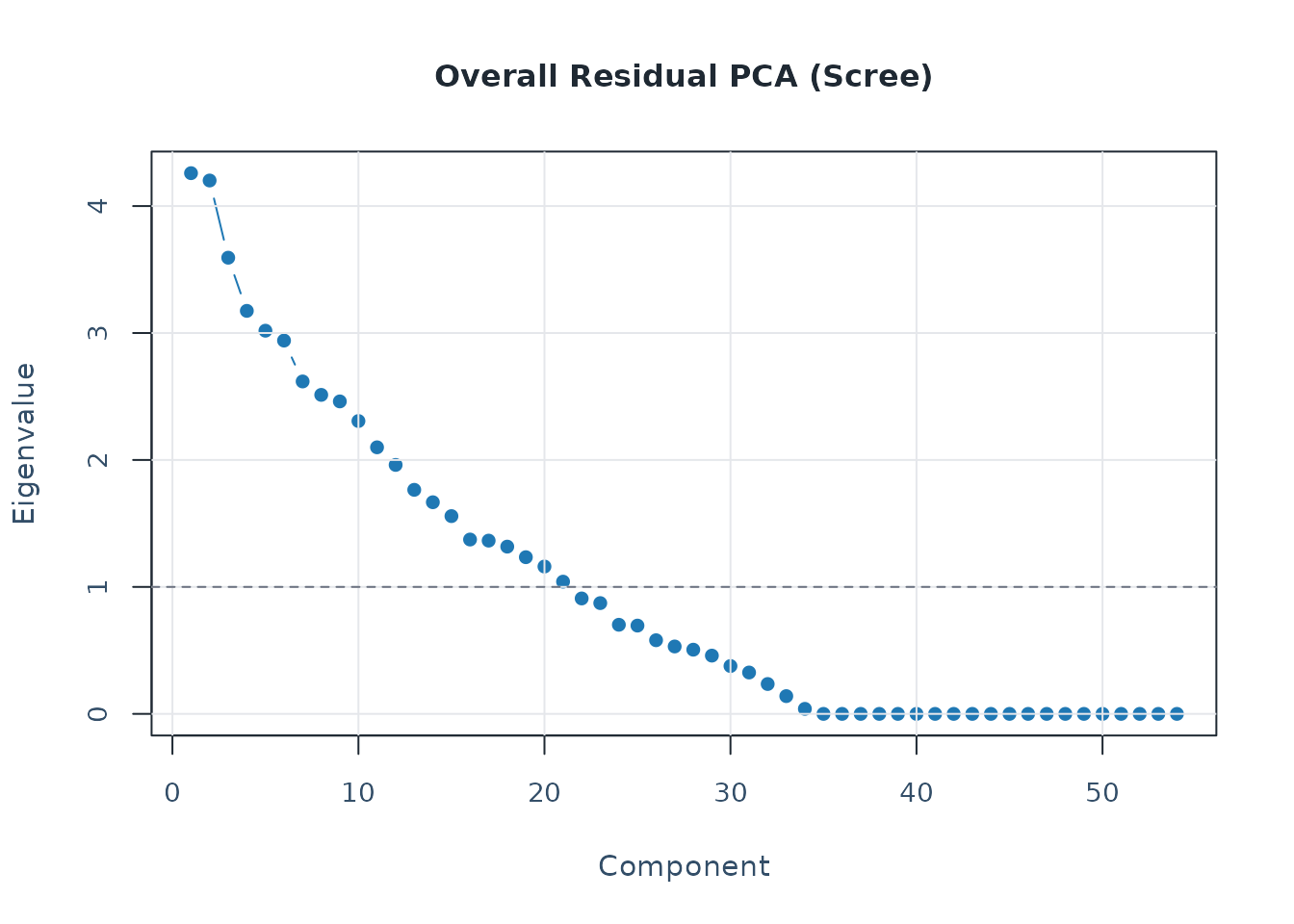
data("mfrmr_example_bias", package = "mfrmr")
bias_df <- mfrmr_example_bias
fit_bias <- fit_mfrm(
  bias_df,
  person = "Person",
  facets = c("Rater", "Criterion"),
  score = "Score",
  method = "MML",
  model = "RSM",
  quad_points = 7
)
diag_bias <- diagnose_mfrm(fit_bias, residual_pca = "none")
bias <- estimate_bias(fit_bias, diag_bias, facet_a = "Rater", facet_b = "Criterion")
fixed <- build_fixed_reports(bias)
apa <- build_apa_outputs(fit_bias, diag_bias, bias_results = bias)

mfrm_threshold_profiles()
#> $profiles
#> $profiles$strict
#> $profiles$strict$n_obs_min
#> [1] 200
#>
#> $profiles$strict$n_person_min
#> [1] 50
#>
#> $profiles$strict$low_cat_min
#> [1] 15
#>
#> $profiles$strict$min_facet_levels
#> [1] 4
#>
#> $profiles$strict$misfit_ratio_warn
#> [1] 0.08
#>
#> $profiles$strict$missing_fit_ratio_warn
#> [1] 0.15
#>
#> $profiles$strict$zstd2_ratio_warn
#> [1] 0.08
#>
#> $profiles$strict$zstd3_ratio_warn
#> [1] 0.03
#>
#> $profiles$strict$expected_var_min
#> [1] 0.3
#>
#> $profiles$strict$pca_first_eigen_warn
#> [1] 1.5
#>
#> $profiles$strict$pca_first_prop_warn
#> [1] 0.1
#>
#>
#> $profiles$standard
#> $profiles$standard$n_obs_min
#> [1] 100
#>
#> $profiles$standard$n_person_min
#> [1] 30
#>
#> $profiles$standard$low_cat_min
#> [1] 10
#>
#> $profiles$standard$min_facet_levels
#> [1] 3
#>
#> $profiles$standard$misfit_ratio_warn
#> [1] 0.1
#>
#> $profiles$standard$missing_fit_ratio_warn
#> [1] 0.2
#>
#> $profiles$standard$zstd2_ratio_warn
#> [1] 0.1
#>
#> $profiles$standard$zstd3_ratio_warn
#> [1] 0.05
#>
#> $profiles$standard$expected_var_min
#> [1] 0.2
#>
#> $profiles$standard$pca_first_eigen_warn
#> [1] 2
#>
#> $profiles$standard$pca_first_prop_warn
#> [1] 0.1
#>
#>
#> $profiles$lenient
#> $profiles$lenient$n_obs_min
#> [1] 60
#>
#> $profiles$lenient$n_person_min
#> [1] 20
#>
#> $profiles$lenient$low_cat_min
#> [1] 5
#>
#> $profiles$lenient$min_facet_levels
#> [1] 2
#>
#> $profiles$lenient$misfit_ratio_warn
#> [1] 0.15
#>
#> $profiles$lenient$missing_fit_ratio_warn
#> [1] 0.3
#>
#> $profiles$lenient$zstd2_ratio_warn
#> [1] 0.15
#>
#> $profiles$lenient$zstd3_ratio_warn
#> [1] 0.08
#>
#> $profiles$lenient$expected_var_min
#> [1] 0.1
#>
#> $profiles$lenient$pca_first_eigen_warn
#> [1] 3
#>
#> $profiles$lenient$pca_first_prop_warn
#> [1] 0.2
#>
#>
#>
#> $pca_reference_bands
#> $pca_reference_bands$eigenvalue
#> critical_minimum          caution           common           strong
#>              1.4              1.5              2.0              3.0
#>
#> $pca_reference_bands$proportion
#>   minor caution  strong
#>    0.05    0.10    0.20
#>
#>
#> attr(,"class")
#> [1] "mfrm_threshold_profiles" "list"
vis <- build_visual_summaries(fit_bias, diag_bias, threshold_profile = "standard")
vis$warning_map$residual_pca_overall
#> [1] "Threshold profile: standard (PC1 EV >= 2.0, variance >= 10%)."
#> [2] "Heuristic reference bands: EV >= 1.4 (critical minimum), >= 1.5 (caution), >= 2.0 (common), >= 3.0 (strong); variance >= 5% (minor), >= 10% (caution), >= 20% (strong)."
#> [3] "Current exploratory PC1 checks: EV>=1.5:Y, EV>=2.0:Y, EV>=3.0:Y, Var>=10%:Y, Var>=20%:Y."
#> [4] "Overall residual PCA PC1 exceeds the current heuristic eigenvalue band (3.22)."
#> [5] "Overall residual PCA PC1 explains 20.1% variance."
The same example_bias dataset also carries a
Group variable so DIF-oriented examples can show a non-null
pattern instead of a fully clean result. It can be loaded either with
load_mfrmr_data("example_bias") or
data("mfrmr_example_bias", package = "mfrmr").
Human-Readable Reporting API
spec <- specifications_report(fit, title = "Study run")
data_qc <- data_quality_report(
  fit,
  data = ej2021_study1,
  person = "Person",
  facets = c("Rater", "Criterion"),
  score = "Score"
)
iter <- estimation_iteration_report(fit, max_iter = 8)
subset_rep <- subset_connectivity_report(fit, diagnostics = diag)
facet_stats <- facet_statistics_report(fit, diagnostics = diag)
cat_structure <- category_structure_report(fit, diagnostics = diag)
cat_curves <- category_curves_report(fit, theta_points = 101)
bias_rep <- bias_interaction_report(bias, top_n = 20)
plot_bias_interaction(bias_rep, plot = "scatter")
Design Simulation and Prediction
The package also supports a separate simulation/prediction layer. The key distinction is:
-
evaluate_mfrm_design()andpredict_mfrm_population()are design-level helpers that summarize expected operating characteristics under an explicit simulation specification. -
predict_mfrm_units()andsample_mfrm_plausible_values()score future or partially observed persons under a fixedMMLcalibration.
sim_spec <- build_mfrm_sim_spec(
  n_person = 30,
  n_rater = 4,
  n_criterion = 4,
  raters_per_person = 2,
  assignment = "rotating"
)

pred_pop <- predict_mfrm_population(
  sim_spec = sim_spec,
  reps = 2,
  maxit = 10,
  seed = 1
)
#> Warning: Optimizer did not fully converge (code = 1). Consider increasing maxit
#> (current: 10) or relaxing reltol (current: 1e-06).
#> Warning: Optimizer did not fully converge (code = 1). Consider increasing maxit
#> (current: 10) or relaxing reltol (current: 1e-06).

summary(pred_pop)$forecast[, c("Facet", "MeanSeparation", "McseSeparation")]
#> # A tibble: 3 × 3
#>   Facet     MeanSeparation McseSeparation
#>   <chr>              <dbl>          <dbl>
#> 1 Criterion          1.87           0.076
#> 2 Person             2.03           0.027
#> 3 Rater              0.728          0.728

keep_people <- unique(toy$Person)[1:18]
toy_mml <- suppressWarnings(
  fit_mfrm(
    toy[toy$Person %in% keep_people, , drop = FALSE],
    person = "Person",
    facets = c("Rater", "Criterion"),
    score = "Score",
    method = "MML",
    quad_points = 5,
    maxit = 15
  )
)

new_units <- data.frame(
  Person = c("NEW01", "NEW01"),
  Rater = unique(toy$Rater)[1],
  Criterion = unique(toy$Criterion)[1:2],
  Score = c(2, 3)
)

pred_units <- predict_mfrm_units(toy_mml, new_units, n_draws = 0)
pv_units <- sample_mfrm_plausible_values(toy_mml, new_units, n_draws = 2, seed = 1)

summary(pred_units)$estimates[, c("Person", "Estimate", "Lower", "Upper")]
#> # A tibble: 1 × 4
#>   Person Estimate Lower Upper
#>   <chr>     <dbl> <dbl> <dbl>
#> 1 NEW01    -0.097 -1.36  1.36
summary(pv_units)$draw_summary[, c("Person", "Draws", "MeanValue")]
#> # A tibble: 1 × 3
#>   Person Draws MeanValue
#>   <chr>  <dbl>     <dbl>
#> 1 NEW01      2         0