
plot_data() is a small accessor for users who want to build custom
base-R, ggplot2, plotly, or table-based displays from mfrmr plot helpers.
It accepts an existing mfrm_plot_data object, or any mfrmr object whose
plot() method supports draw = FALSE. Use plot_data_components() first
when you want to inspect which components are available before extracting
one.
Titles, subtitles, and explanatory footnotes are omitted from figures by
default. Use plot_data(p, "title") for the suggested title and
plot_data(p, "notes") for a Type/Text table of descriptions and cautions.
This works for saved 0.2.x plot payloads and mfrmr-generated ggplots,
including after saveRDS()/readRDS(). Printing an mfrm_plot_data object
also displays its notes in the console. Axes, legends, panel headings and
data/status symbols remain in the figure. Removing figure text does not
remove numerical warnings or strengthen the interpretation of a result.
Usage
plot_data(
  x,
  component = NULL,
  type = NULL,
  ...,
  format = c("native", "long"),
  value_cols = NULL
)
Arguments
- x
An
mfrm_plot_dataobject, or a fitted/report/review object with aplot(..., draw = FALSE)method.- component
Optional single component name inside the reusable plot data. When
NULL, the full plot-data list is returned.- type
Optional plot type passed to
plot()whenxis not already anmfrm_plot_dataobject.- ...
Additional arguments passed to
plot(..., draw = FALSE)whenxis not already anmfrm_plot_dataobject.- format
"native"(default) returns the saved component unchanged."long"reshapes a selected table or matrix without dropping missing cells.- value_cols
Explicit table columns to gather into
VariableandValue. Other columns, and an addedSourceRow, remain identifiers/metadata. Select compatible value types and comparable units; estimates, standard errors and interval bounds are distinct quantities, not replicate draws. Matrices instead yield Row, Column, RowLabel, ColumnLabel and Value, with indices retaining identity even if labels repeat. Already-long tables (including cluster-profileobservations) need no reshaping.
Custom distribution plots
A cluster profile's observations component contains one row per original
entity and selected feature, with ID, Feature, Value, Cluster, Included and
MissingReason. Missing values and omitted entities remain. Use Included to
select the plotted population explicitly. table is the summary, not raw
observations. Export either with write.csv; use the observations for custom
box/violin/raincloud plots. Feature units are the original units, supplied by
the study. A smooth density is usually inappropriate for a few ordinal bins.
online networks and reporting guide demonstrates custom plots and CSVs.
Examples
library(mfrmr)
# Saved synthetic MML/RSM analysis of example_operational.
# For your own data, fit a model first; see ?fit_mfrm.
example_fit <- readRDS(system.file("examples", "operational-mml.rds", package = "mfrmr"))
fit <- example_fit$fit
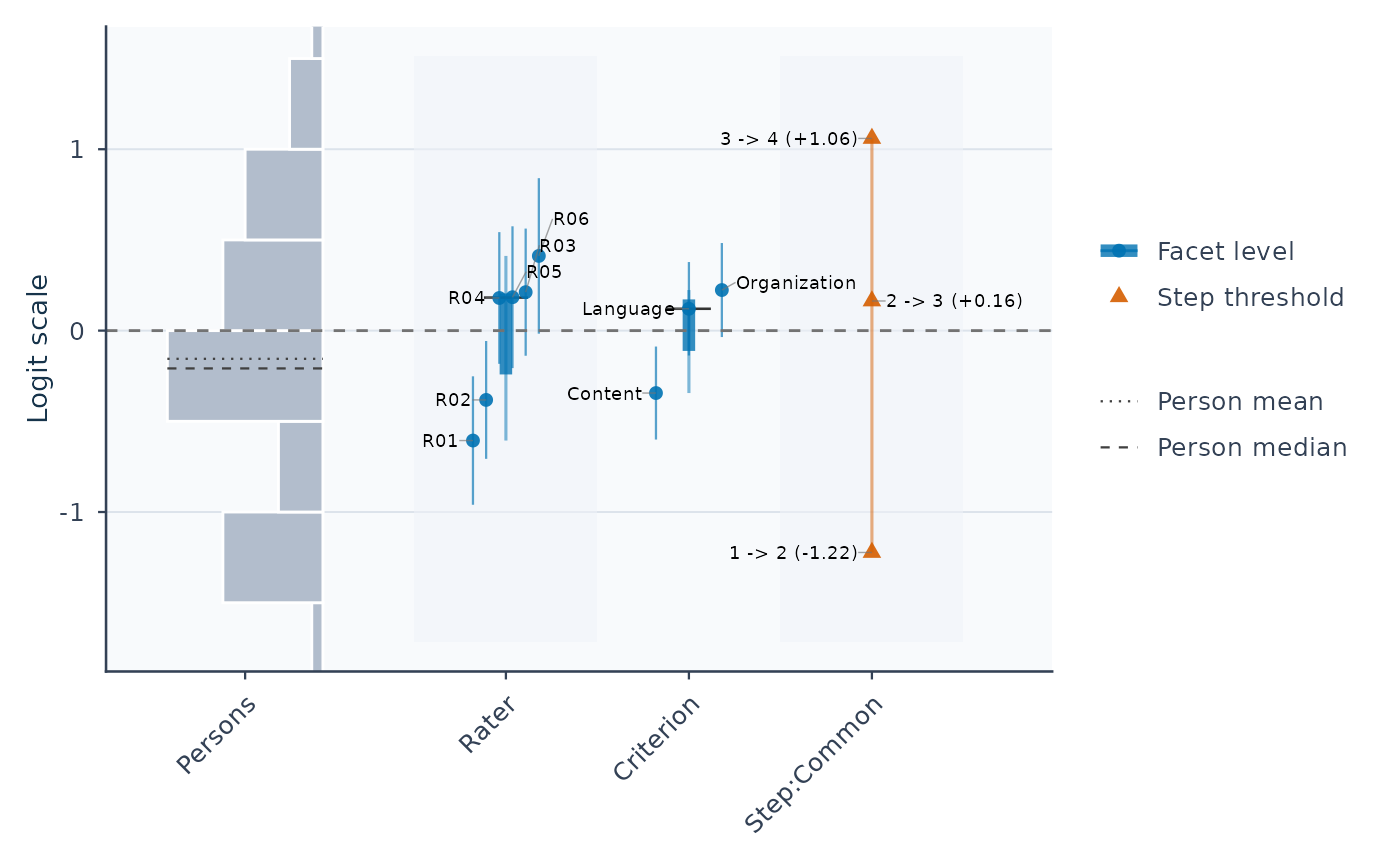
# Draw the Wright map and keep its reusable data
wright <- plot(fit)
 plot_data(wright, "notes")
#> Type
#> 1 interpretation
#> 2 description
#> 3 display
#> 4 score_coding
#> 5 orientation
#> 6 orientation
#> 7 orientation
#> 8 step
#> Text
#> 1 Stored fit readiness plus numerical, data-support, connectivity, and stability checks passed. Treat this display as diagnostic evidence, not automatic publication approval.
#> 2 Shared logit scale for persons, facets, and thresholds
#> 3 Persons: N=48; mean=-0.16; median=-0.21.
#> 4 Score meaning is supplied by the rubric: higher coded scores need not mean better performance. Reversing category labels alone does not reverse the fitted scale.
#> 5 Higher Person locations increase expected coded scores in these positive-discrimination models, holding other effects fixed.
#> 6 Rater: higher locations reduce expected coded scores, holding other effects fixed.
#> 7 Criterion: higher locations reduce expected coded scores, holding other effects fixed.
#> 8 A Step describes the transition between adjacent score categories, not a learning stage or a pass/fail cut. At the corresponding predictor value, the two categories have equal probability, not necessarily probability 0.5 each. Stored step offsets and full ability-axis crossings differ when other facet effects or interactions are included; check the reference profile and step owner.
# Extract the plotted locations as a table
locations <- plot_data(wright, component = "locations")
head(locations)
#> # A tibble: 6 × 39
#> Group Label PlotType Estimate SE Fixed CI_Level SE_Method PrecisionTier
#> <fct> <chr> <chr> <dbl> <dbl> <lgl> <dbl> <chr> <chr>
#> 1 Rater R01 Facet level -0.606 0.181 FALSE 0.95 Observati… exploratory
#> 2 Rater R02 Facet level -0.382 0.166 FALSE 0.95 Observati… exploratory
#> 3 Rater R04 Facet level 0.180 0.185 FALSE 0.95 Observati… exploratory
#> 4 Rater R05 Facet level 0.184 0.199 FALSE 0.95 Observati… exploratory
#> 5 Rater R03 Facet level 0.212 0.179 FALSE 0.95 Observati… exploratory
#> 6 Rater R06 Facet level 0.412 0.219 FALSE 0.95 Observati… exploratory
#> # ℹ 30 more variables: SupportsFormalInference <lgl>, SEUse <chr>,
#> # CIBasis <chr>, CIUse <chr>, CIEligible <lgl>, CILabel <chr>,
#> # Measure_Source <chr>, CI_Lower <dbl>, CI_Upper <dbl>, Step <chr>,
#> # StepIndex <int>, BoundarySeparated <lgl>, Highlighted <lgl>, XBase <dbl>,
#> # X <dbl>, OriginalEstimate <dbl>, BelowRange <lgl>, AboveRange <lgl>,
#> # DisplayEstimate <dbl>, DisplayLabel <chr>, OriginalCI_Lower <dbl>,
#> # OriginalCI_Upper <dbl>, DisplayCI_Lower <dbl>, DisplayCI_Upper <dbl>, …
# For table extraction alone, no graphics device is needed
locations_only <- plot_data(fit, component = "locations")
head(locations_only)
#> # A tibble: 6 × 39
#> Group Label PlotType Estimate SE Fixed CI_Level SE_Method PrecisionTier
#> <fct> <chr> <chr> <dbl> <dbl> <lgl> <dbl> <chr> <chr>
#> 1 Rater R01 Facet level -0.606 0.181 FALSE 0.95 Observati… exploratory
#> 2 Rater R02 Facet level -0.382 0.166 FALSE 0.95 Observati… exploratory
#> 3 Rater R04 Facet level 0.180 0.185 FALSE 0.95 Observati… exploratory
#> 4 Rater R05 Facet level 0.184 0.199 FALSE 0.95 Observati… exploratory
#> 5 Rater R03 Facet level 0.212 0.179 FALSE 0.95 Observati… exploratory
#> 6 Rater R06 Facet level 0.412 0.219 FALSE 0.95 Observati… exploratory
#> # ℹ 30 more variables: SupportsFormalInference <lgl>, SEUse <chr>,
#> # CIBasis <chr>, CIUse <chr>, CIEligible <lgl>, CILabel <chr>,
#> # Measure_Source <chr>, CI_Lower <dbl>, CI_Upper <dbl>, Step <chr>,
#> # StepIndex <int>, BoundarySeparated <lgl>, Highlighted <lgl>, XBase <dbl>,
#> # X <dbl>, OriginalEstimate <dbl>, BelowRange <lgl>, AboveRange <lgl>,
#> # DisplayEstimate <dbl>, DisplayLabel <chr>, OriginalCI_Lower <dbl>,
#> # OriginalCI_Upper <dbl>, DisplayCI_Lower <dbl>, DisplayCI_Upper <dbl>, …