
Choose the result you need
Start with the intended score and decision, then choose a branch. These are connected workflows, not a checklist requiring every analysis.
| Your situation | Connected route | What to carry into the report |
|---|---|---|
| Define what was rated and whether the design links the groups |
describe_mfrm_data() → model/design review →
subset_connectivity_report() or
build_mfrm_network_review() after fitting |
Rubric endpoints, rating unit, assigned/missing rows, shared observations and identification checks. A connected graph alone does not establish a common scale. |
| Estimate person measures and named rater/criterion effects |
fit_mfrm() → summary() →
diagnose_mfrm() and eligible intervals →
mfrm_results() → mfrm_report()
|
Model, scale, estimates, uncertainty, Separation/Strata/Reliability, fit and the figures that answer the question. |
| Decide how many raters or tasks a score needs |
mfrm_g_study() → mfrm_d_study() →
plot() / summary() → eligible plan
comparisons |
G/D-study components, score weights, G/Phi/SEM, future counts and uncertainty. No MFRM fit is required. |
| Describe observed agreement | Match the rating unit → pairwise_kappa_table(),
krippendorff_alpha_table() or
pairwise_icc_table()
|
Agreement target, category distances/ICC definition, overlap and exclusions. Choose the coefficient from the question. |
| Reuse a scale across forms or waves | Anchor review → anchored fit / linking review → drift and eligible uncertainty | Anchor provenance and scale, invariance assumption, fixed versus propagated uncertainty. A common label is not a common calibration. |
| Investigate an unexpected rater/criterion combination or group contrast | Diagnostics → specified estimate_bias() or
analyze_dff() → signed tables and plot() →
reporting |
Bias/DFF target, cell counts, direction, multiplicity and conditional uncertainty; a screen does not establish unfairness. |
| Decide whether another model changes the answer | Matched fits → compare_mfrm() →
build_model_choice_review() →
build_summary_table_bundle()
|
Model comparison, comparable likelihoods, eligible tests and changes in substantive conclusions. |
| Investigate structure left unexplained or describe groups | Residual diagnostics / analyze_residual_pca() /
q3_statistic() → mfrm_residual_network() →
mfrm_report(); separately, declared entity features →
clustering |
Residual exploration and feature groups have different inputs. Retain overlap, feature construction and exploratory status. |
| Give feedback, score new responses or save evidence | Eligible rater report / score_mfrm_persons() or
portable calibration → plots, export and RDS |
Recipient-specific evidence and limitations, scoring prior/calibration version and the source of uncertainty. See the reporting map. |
Before any branch, record the meaning of low and high
scores. A column named Comprehensibility may encode ease or
difficulty. Higher Person locations predict higher coded categories;
they do not inherently mean better performance. With the default Rater
orientation, higher locations predict lower coded scores. See score
direction before interpreting severity, bias, plots or anchors.
Changing positive_facets is not reverse-coding the
outcome.
If Content and Organization are separate reported scores, start with the criterion-versus-score distinction. A Criterion facet in one-dimensional MFRM does not estimate a separate ability for each criterion. Multivariate G theory estimates cross-score covariance components; it does not fit multidimensional IRT.
Put the network at the stage its edges describe
| Network | Best point in the workflow | What an edge means |
|---|---|---|
| Assignment/co-observation | Design review, before interpreting measures; return to it when planning additional links or anchors | Who shares observed ratings: mfrm_network_analysis() →
build_mfrm_network_review(). Pass data,
person, facets, score before
fitting; use basis = "planned" without a score column for
an assignment roster. Inspect the person-rater projection as well as the
full graph. |
| Rater score relations | After matching shared responses, alongside agreement and rater feedback | Observed score agreement/disagreement or directional differences in
rater_network_analysis(); cross-criterion observed
correlations in rater_halo_network_analysis(). These are
not residual networks or causal halo tests. |
| Residual associations or communities | After fitting and checking residual/overlap definitions, for a stated unexplained-structure question | Associations left after the model.
mfrm_residual_network() supplies signed residual
correlations and optional hierarchical groups. Report all pairs, overlap
and missingness with mfrm_report(). This is descriptive
exploration, not EGA or a jointly fitted network model. |
An assignment graph is especially useful for explaining why adding a shared performance or rater might improve linking. It cannot create direct pairwise agreement evidence where no common responses were rated. Feature clustering can describe external rater backgrounds; clustering estimated bias or residual profiles additionally needs explicit aggregation, missingness, comparability and estimation-uncertainty treatment. The current feature API does not supply those steps automatically.
Quick start
By the end of this lesson you should be able to prepare one-rating-per-row data, estimate abilities and facet effects, identify results needing review, and save an analysis with its assumptions. Start with the synthetic example, then adapt the CSV lesson. Follow-up analyses are optional and should answer your assessment question.
Use this reading route:
| What you need now | Where to go |
|---|---|
| Choose a model and estimator for your purpose | Model and estimator choice, including when greater complexity helps and when it does not |
| Run and understand a first analysis | Quick start, including individual estimates and review messages below |
| Analyze your own rating sheet | Use your own CSV, including stopped checks and wide-to-long reshaping |
| Interpret fit, precision and rater feedback | Continue with diagnostics and reporting |
| Find the calculation and its research basis |
help("mfrmr_methods_reference"), then the linked
function’s method and References sections |
This tutorial follows the ordinary fixed-facet
fit_mfrm() workflow. To plan the number of tasks or raters
for an observed score, use Plan an
assessment with G theory; no MFRM fit is required for that workflow.
To choose between fixed facets, shared random raters and Person-specific
testlets, use mfrmr_output_guide("models") or
help("mfrmr_workflow_methods"). The extended models have
dedicated tutorials: Shared
random raters: feedback and replacement raters and Dependent
ratings within a person: testlet models. Their prediction targets
and reporting support differ. The diagnostics and reports below follow
ordinary RSM/PCM fits. Two-family GPCM and corrected JML also have class
mfrm_fit, but require their model-specific result routes;
sharing that class does not make these ordinary diagnostics available.
See mfrmr_output_guide("gpcm_capabilities") and GPCM
scope and current limitations before changing model family.
This example estimates person abilities while accounting for rater
severity and criterion difficulty. A facet is a source of
variation in scores; here, Rater and Criterion
are facets, and individual raters and criteria are their
levels. The data are synthetic, with one row per rating and
scores from 1 to 4.
The example data are included in the package. The loading line below
creates ratings; you do not need to prepare a file or
construct the scores first. head(ratings) shows the first
six rows. The quoted column names in fit_mfrm() are
case-sensitive; Study and Group are extra
labels unused by this model. MML selects marginal maximum
likelihood; RSM selects a rating-scale model with shared
category thresholds (the transitions between adjacent scores). The
rubric uses scores 1 through 4.
category_policy = "preserve" keeps that category ladder; it
prevents an unobserved intermediate category from being silently
collapsed into a different scale.
# Load the package
library(mfrmr)

# Load example ratings and look at the first six rows
ratings <- load_mfrmr_data("example_operational")
head(ratings)
#>                Study Person Rater    Criterion Score Group
#> 1 OperationalExample   P001   R01     Language     4     A
#> 2 OperationalExample   P001   R01 Organization     2     A
#> 3 OperationalExample   P001   R02      Content     4     A
#> 4 OperationalExample   P001   R02     Language     3     A
#> 5 OperationalExample   P001   R02 Organization     2     A
#> 6 OperationalExample   P002   R01      Content     3     A

# Fit the model
fit <- fit_mfrm(
  data = ratings,
  person = "Person",
  facets = c("Rater", "Criterion"),
  score = "Score",
  rating_min = 1, rating_max = 4,
  category_policy = "preserve",
  method = "MML",
  model = "RSM"
)

# Plot the results (Wright map)
plot(fit)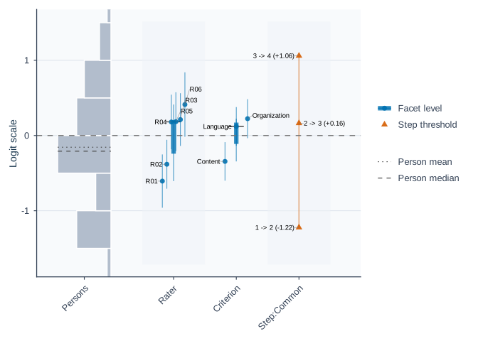
# Save the summary, then display its tables
results <- summary(fit)
results$person_overview # One row summarizing person ability estimates
#> # A tibble: 1 × 11
#> Persons DistributionN ReviewExcludedExtremeE…¹ EstimateUse Mean SD Median
#> <int> <int> <int> <chr> <dbl> <dbl> <dbl>
#> 1 48 48 0 source_fit… -0.155 0.824 -0.208
#> # ℹ abbreviated name: ¹ReviewExcludedExtremeEAPs
#> # ℹ 4 more variables: Min <dbl>, Max <dbl>, Span <dbl>, MeanPosteriorSD <dbl>
results$facet_overview # One row per facet: number of levels, mean, SD, range
#> # A tibble: 2 × 7
#> Facet Levels MeanEstimate SDEstimate MinEstimate MaxEstimate Span
#> <chr> <int> <dbl> <dbl> <dbl> <dbl> <dbl>
#> 1 Criterion 3 0 0.302 -0.344 0.224 0.568
#> 2 Rater 6 -4.64e-18 0.399 -0.606 0.412 1.02
# Check the interpretation status and recommended next step
results$decision
#> Interpretation
#> 1 Fit-readiness requirements satisfied; formal precision review required
#> FormalInference FitReadiness
#> 1 No ready
#> Why
#> 1 Formal precision support has not been evaluated. These checks assess numerical readiness and the requested precision method under the specified model; they do not establish model adequacy or finite-sample coverage for this design.
#> NextAction
#> 1 Run `diagnose_mfrm()` and pass its result as `diagnostics =` to evaluate formal precision support; fit readiness alone is not a formal-inference decision.<- saves an object without printing it. Here
ratings holds the data, fit holds the model,
and results holds its summary. $ selects a
named part: results$person_overview displays just that
table. Enter results to print the full summary.
The Wright map displays the estimates in logits, the model’s measurement units, rather than the original 1-to-4 scores. With this example’s default orientation, higher person estimates mean higher ability; higher rater estimates mean more severe ratings, and higher criterion estimates mean greater difficulty.
The native models use the logistic metric (L-metric), with D
= 1: there is no extra 1.7 or 1.702 normal-ogive approximation
factor. In this RSM example, an ability increase of one unit raises each
adjacent-category log odds by one, holding other parameters fixed. For
GPCM, the effective discrimination multiplies that change. A normal
ability distribution is a separate assumption and does not change the
response link. See ?fit_mfrm for scale conventions.
The overview tables describe distributions:
person_overview has one row for all 48 persons, and
facet_overview has one row for each facet.
Mean/MeanEstimate is the average,
SD/SDEstimate is the spread, and
Min/Max or
MinEstimate/MaxEstimate give the endpoints.
Rater and criterion means are constrained to zero here; their SDs and
ranges show differences among levels.
Inspect individual estimates
estimates <- as.data.frame(fit)
head(subset(estimates, Facet == "Person")) # First six persons
#>    Facet Level    Estimate Extreme
#> 1 Person  P001  0.28429588    none
#> 2 Person  P002  0.66118004    none
#> 3 Person  P003  0.02177773    none
#> 4 Person  P004  0.22410785    none
#> 5 Person  P005 -0.17496065    none
#> 6 Person  P006  0.67681003    none
subset(estimates, Facet == "Rater")       # All raters
#>    Facet Level   Estimate Extreme
#> 49 Rater   R01 -0.6059776    <NA>
#> 50 Rater   R02 -0.3820356    <NA>
#> 51 Rater   R03  0.2120388    <NA>
#> 52 Rater   R04  0.1799462    <NA>
#> 53 Rater   R05  0.1842365    <NA>
#> 54 Rater   R06  0.4117917    <NA>
subset(estimates, Facet == "Criterion")   # All criteria
#>        Facet        Level   Estimate Extreme
#> 55 Criterion      Content -0.3441471    <NA>
#> 56 Criterion     Language  0.1204520    <NA>
#> 57 Criterion Organization  0.2236950    <NA>
Facet identifies the type of estimate,
Level identifies the person, rater, or criterion, and
Estimate is its value in logits.
Check what needs review
Read results$decision, especially Why and
NextAction, before interpreting or reporting estimates.
FormalInference = "No" in this first summary can mean that
precision has not yet been reviewed; it does not necessarily mean that
fitting failed. The default summary does not compute diagnostics.
diagnostics <- diagnose_mfrm(fit)
diagnostic_summary <- summary(diagnostics)
diagnostic_summary$decision
#>               Interpretation FormalInference FitReadiness
#> 1 Ready for formal inference             Yes        ready
#>                                                                                                                                                                                                                                 Why
#> 1 All stored fit-readiness components passed. These checks assess numerical readiness and the requested precision method under the specified model; they do not establish model adequacy or finite-sample coverage for this design.
#>                                                                                            NextAction
#> 1 Inspect `diagnostic_basis` before comparing legacy residual evidence with strict marginal evidence.
For your own data, follow Use your own
CSV below. For reporting,
res <- mfrm_results(fit, diagnostics = diagnostics)
builds a comprehensive object that reuses the checks above. Pass
res to mfrm_report() or
export_mfrm_results(); results remains the
basic summary.
Use your own CSV
The goal here is to estimate person ability while accounting for rater severity and criterion difficulty in your own ratings. Start with the same row layout as the packaged example: one score from one rater for one person on one criterion. For example:
| Person | Rater | Criterion | Score |
|---|---|---|---|
| 001 | R1 | Content | 3 |
| 001 | R1 | Style | 2 |
| 001 | R2 | Content | 4 |
| 001 | R2 | Style | 3 |
The repeated 001 is intentional: all four scores belong
to the same person. Keep IDs consistent across rows. These four rows
explain the layout; use the complete set of ratings for estimation.
Score contains the ordered integer categories from the
rubric, not totals or averages across raters. This example uses two
non-person facets; choose facets that represent your design.
1. Read and inspect the file
You can practice the full workflow without supplying a file. This block writes the packaged synthetic ratings to a new temporary CSV:
library(mfrmr)
csv_path <- tempfile(fileext = ".csv")
write.csv(load_mfrmr_data("example_operational"), csv_path,
          row.names = FALSE, na = "")
For your own data, export your rating sheet as CSV UTF-8, with column names in the first row. Skip the practice block above and select your file instead:
library(mfrmr)
csv_path <- file.choose()
For a reusable script, replace file.choose() with a
quoted path such as "data/ratings.csv", relative to the
folder shown by getwd(). Both routes now use the same
import and analysis code:
ratings <- read.csv(
  csv_path,
  colClasses = "character",
  na.strings = "",
  check.names = FALSE,
  fileEncoding = "UTF-8-BOM"
)
# Treat the documented missing-score marker only in the score column
ratings <- recode_missing_codes(ratings, columns = "Score", codes = "NA")
head(ratings)
#>                Study Person Rater    Criterion Score Group
#> 1 OperationalExample   P001   R01     Language     4     A
#> 2 OperationalExample   P001   R01 Organization     2     A
#> 3 OperationalExample   P001   R02      Content     4     A
#> 4 OperationalExample   P001   R02     Language     3     A
#> 5 OperationalExample   P001   R02 Organization     2     A
#> 6 OperationalExample   P002   R01      Content     3     A
names(ratings)
#> [1] "Study"     "Person"    "Rater"     "Criterion" "Score"     "Group"
table(ratings$Score, useNA = "ifany")
#>
#>  1  2  3  4
#> 62 96 78 46
Reading columns as text preserves distinct IDs such as
001, 1, and NA;
mfrmr converts numeric score strings such as
"3" for estimation. check.names = FALSE
preserves the headers. Empty cells are missing in every column; the
literal marker NA is recoded only in Score.
Use the missing-score markers declared for your data. Zero is a score
when the rubric includes zero, and must not be used to fill unassigned
rating cells.
The quoted column names in the next two steps must match
names(ratings), including capitalization and spaces. You do
not have to rename your file’s columns. For headers
Student, Judge, Task, and
Rating, change the arguments in both
describe_mfrm_data() and fit_mfrm() as
follows:
| Argument | Four-column example | Your alternative headers |
|---|---|---|
person |
"Person" |
"Student" |
facets |
c("Rater", "Criterion") |
c("Judge", "Task") |
score |
"Score" |
"Rating" |
Also use columns = "Rating" in the recoding call and
inspect ratings$Rating instead of
ratings$Score. Extra columns such as the practice file’s
Study and Group are unused by this model.
2. Review the rows and the rubric
Set the minimum and maximum from the rubric, not the
observed minimum and maximum in this sample. The code below describes a
1-to-4 rubric. Keep the same values in the data review and the fit.
category_policy = "preserve" preserves the intended
category structure, including categories with no observations.
data_review <- describe_mfrm_data(
  data = ratings,
  person = "Person",
  facets = c("Rater", "Criterion"),
  score = "Score",
  rating_min = 1,
  rating_max = 4,
  category_policy = "preserve"
)
data_review$row_retention
#>                             Stage Rows DroppedRows
#> 1          input_selected_columns  282           0
#> 2 after_missing_and_weight_filter  282           0
#>                            DroppedReason
#> 1
#> 2 missing values or non-positive weights
data_review$missing_by_column
#> # A tibble: 4 × 2
#>   Column    Missing
#>   <chr>       <int>
#> 1 Person          0
#> 2 Rater           0
#> 3 Criterion       0
#> 4 Score           0
data_review$score_distribution
#> # A tibble: 4 × 4
#>   Score  RawN WeightedN Percent
#>   <int> <int>     <dbl>   <dbl>
#> 1     1    62        62    22.0
#> 2     2    96        96    34.0
#> 3     3    78        78    27.7
#> 4     4    46        46    16.3
data_review$design_connectivity
#>      Basis     Facet PersonNodes FacetLevelNodes Edges Components
#> 1 observed     Rater          48               6    96          1
#> 2 observed Criterion          48               3   144          1
#>   LargestComponentPersons LargestComponentLevels LargestComponentPercent
#> 1                      48                      6                     100
#> 2                      48                      3                     100
#>   Connected
#> 1      TRUE
#> 2      TRUE
Read these four tables in order:
-
row_retention: compare input and retainedRows; inspect anyDroppedRows. A missing score or required ID removes that rating row, not automatically the person’s other ratings. The package does not fill missing ratings. -
missing_by_column: locate missing input values. Non-numeric score text can also cause row loss; inspect warnings anddata_review$preparation_noteswhen the retained count is unexpected. -
score_distribution:RawNcounts the retained ratings in each category. A zero count in an internal category, such as 3 on a 1-to-4 scale, prevents fitting withcategory_policy = "preserve". Review the data and rubric before changing categories; increasing optimizer iterations cannot supply missing category information. -
design_connectivity:Components = 1means a facet’s levels are connected through shared persons. More than one component needs design review before comparing levels across components. Connectivity alone does not establish full model identification.
For the practice CSV, all 282 input rows are retained, all four
categories have observations, and each facet has one connected
component. Six planned ratings are absent from the file; column missing
counts cannot detect absent rows. If you have a planned assignment
roster, pass it as expected_design to
describe_mfrm_data() to assess these omissions. The applied
example later in this vignette shows how. Without a roster, structural
missingness is reported as not assessed; a complete
person-by-rater-by-criterion crossing is not assumed.
3. Fit and read the results
After resolving the data-review findings, fit the same rows, columns, and rubric. This example uses an RSM with shared category thresholds; the choice should reflect the scoring design. Diagnostics then supply evidence for the interpretation decision.
csv_fit <- fit_mfrm(
  data = ratings,
  person = "Person",
  facets = c("Rater", "Criterion"),
  score = "Score",
  rating_min = 1,
  rating_max = 4,
  category_policy = "preserve",
  method = "MML",
  model = "RSM"
)
csv_diagnostics <- diagnose_mfrm(csv_fit)
csv_results <- summary(csv_fit, diagnostics = csv_diagnostics)
csv_results$decision
#>               Interpretation FormalInference FitReadiness
#> 1 Ready for formal inference             Yes        ready
#>                                                                                                                                                                                                                                 Why
#> 1 All stored fit-readiness components passed. These checks assess numerical readiness and the requested precision method under the specified model; they do not establish model adequacy or finite-sample coverage for this design.
#>                                                                                                                                                                   NextAction
#> 1 After reviewing convergence, run `review <- summary(fit, profile = "facets", detail = "brief")` for the comprehensive measurement review; FACETS software is not required.
Read Why and NextAction before using the
estimates. A FormalInference value of "No"
means that the stated obstacle to formal use still needs attention.
Diagnostic plots can help investigate it. Even a supported precision
decision does not establish the validity of the assessment or answer the
study’s substantive question.
plot(csv_fit)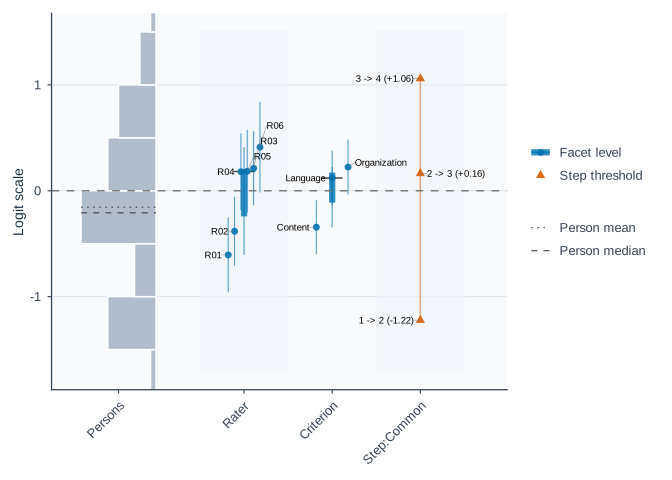
csv_estimates <- as.data.frame(csv_fit)
head(subset(csv_estimates, Facet == "Person"))
#>    Facet Level    Estimate Extreme
#> 1 Person  P001  0.28429588    none
#> 2 Person  P002  0.66118004    none
#> 3 Person  P003  0.02177773    none
#> 4 Person  P004  0.22410785    none
#> 5 Person  P005 -0.17496065    none
#> 6 Person  P006  0.67681003    none
subset(csv_estimates, Facet == "Rater")
#>    Facet Level   Estimate Extreme
#> 49 Rater   R01 -0.6059776    <NA>
#> 50 Rater   R02 -0.3820356    <NA>
#> 51 Rater   R03  0.2120388    <NA>
#> 52 Rater   R04  0.1799462    <NA>
#> 53 Rater   R05  0.1842365    <NA>
#> 54 Rater   R06  0.4117917    <NA>
subset(csv_estimates, Facet == "Criterion")
#>        Facet        Level   Estimate Extreme
#> 55 Criterion      Content -0.3441471    <NA>
#> 56 Criterion     Language  0.1204520    <NA>
#> 57 Criterion Organization  0.2236950    <NA>
Level identifies the person, rater, or criterion;
Estimate is the fitted value in logits. With these
defaults, higher person values mean higher ability, higher rater values
mean more severe ratings, and higher criterion values mean greater
difficulty. The rater and criterion estimates are centered at zero
within each facet. In the practice file, R06 is about +0.41 and R01
about -0.61: R06 is estimated to rate more severely after accounting for
person ability and criterion difficulty. This difference alone does not
establish statistical significance.
With custom facet names, change the Facet filters too,
for example from "Rater" to "Judge"; person
rows retain Facet == "Person" even when the input ID column
is named Student. To inspect all persons, remove
head(). The overview tables in csv_results
summarize distributions; the rows in csv_estimates give
individual estimates.
If a check stops you
| What you see | What to check or change |
|---|---|
| The CSV is not found | Use file.choose() or check the quoted path relative to
getwd(). An .xlsx workbook must first be
exported as CSV. |
| All fields appear in one column, or the header is garbled | Check the separator and encoding. Use sep = ";" for a
semicolon-delimited file; re-export as CSV UTF-8 if text is
unreadable. |
Column(s) not found in data |
Compare names(ratings) with the names in
person, facets, and score; check
spelling, spaces, and case. |
| Non-numeric or fractional scores | Check table(ratings$Score, useNA = "ifany"). Map rubric
labels explicitly to their ordered integer codes. Do not round totals or
averaged ratings to make them fit. |
| Scores outside the supplied range, such as 99 | Check whether the value is an error or a documented missing code. Correct the value or recode the declared missing marker; keep the range tied to the rubric. |
| Fewer retained rows than expected | Inspect data_review$missing_by_column and
data_review$preparation_notes. Correct unintended missing
IDs or score values, then rerun the review and fit. |
| Duplicated person-by-facet cells | Inspect data_review$duplicate_cell_detail. Correct
accidental duplicates. If these are distinct tasks or occasions, include
the corresponding facet; do not automatically delete legitimate
ratings. |
| A category has no observations, or the design is disconnected | Review category coding and assignments. Do not invent ratings or change optimizer settings to resolve missing information. |
If your data documentation defines 99 and .
as missing scores, recode only that column before step
2. This preserves an ID such as 99:
ratings <- recode_missing_codes(
  ratings, columns = "Score", codes = c("99", ".")
)
table(ratings$Score, useNA = "ifany")
Use only the codes declared for your data, and change
"Score" if your score column has another name. Then repeat
steps 2 and 3 with the recoded data.
If criteria occupy separate columns
For a sheet with one row per person-rater pair and separate criterion scores, reshape the criterion columns into rating rows:
wide <- data.frame(
  Person = c("001", "001"),
  Rater = c("R1", "R2"),
  Content = c(3, 4),
  Style = c(2, 3)
)
ratings_long <- tidyr::pivot_longer(
  wide,
  cols = c("Content", "Style"),
  names_to = "Criterion",
  values_to = "Score"
)
ratings_long
#> # A tibble: 4 × 4
#>   Person Rater Criterion Score
#>   <chr>  <chr> <chr>     <dbl>
#> 1 001    R1    Content       3
#> 2 001    R1    Style         2
#> 3 001    R2    Content       4
#> 4 001    R2    Style         3
The output is the four-row layout at the start of this section. For
your full sheet, read the CSV into wide, select its actual
criterion columns in cols, and use
ratings <- ratings_long before step 2. Keep the complete
dataset; these four demonstration rows are not sufficient for the
intended analysis.
Continue with diagnostics and reporting
The following sections ask three questions: are the estimates interpretable, what needs closer inspection, and what information belongs in a report? First select the analysis to carry through every table, figure and export. The default uses Quick start, including its known assignment roster:
analysis_data <- ratings
fit_toy <- fit
diag_toy <- diagnostics
data("mfrmr_example_operational_design", package = "mfrmr")
analysis_roster <- mfrmr_example_operational_design
For your CSV, run this replacement block instead. The downstream object names stay the same so the remaining code uses your analysis:
analysis_data <- ratings
fit_toy <- csv_fit
diag_toy <- csv_diagnostics
analysis_roster <- NULL # Replace with your own planned roster if available
Do not use the packaged roster for your own ratings.
NULL means planned omissions cannot be assessed; it does
not mean there are no missing ratings. The numerical examples in the
prose below describe the synthetic data. If your headers or rubric
differ, update person, facets,
score, the rating limits and later
"Rater"/"Criterion" selections as in the CSV
lesson.
1. Check the data and estimation record
data_review_toy <- describe_mfrm_data(
  data = analysis_data,
  person = "Person",
  facets = c("Rater", "Criterion"),
  score = "Score",
  rating_min = 1,
  rating_max = 4,
  category_policy = "preserve",
  expected_design = analysis_roster
)
data_summary_toy <- summary(data_review_toy)
data_summary_toy$structural_missingness
#>     Status ExpectedCells ObservedCells MatchedCells MissingExpectedCells
#> 1 declared           288           282          282                    6
#>   UnexpectedObservedCells CoverageRate ExpectedOnlyPersons UnexpectedPersons
#> 1                       0    0.9791667                   0                 0
data_summary_toy$design_connectivity
#>               Basis     Facet PersonNodes FacetLevelNodes Edges Components
#> 1          observed     Rater          48               6    96          1
#> 2          observed Criterion          48               3   144          1
#> 3 declared_expected     Rater          48               6    96          1
#> 4 declared_expected Criterion          48               3   144          1
#>   LargestComponentPersons LargestComponentLevels LargestComponentPercent
#> 1                      48                      6                     100
#> 2                      48                      3                     100
#> 3                      48                      6                     100
#> 4                      48                      3                     100
#>   Connected
#> 1      TRUE
#> 2      TRUE
#> 3      TRUE
#> 4      TRUE

fit_summary_toy <- summary(fit_toy)
fit_summary_toy$overview[, c("Model", "Method", "N", "Persons", "Converged")]
#> # A tibble: 1 × 5
#>   Model Method     N Persons Converged
#>   <chr> <chr>  <dbl>   <int> <lgl>
#> 1 RSM   MML      282      48 TRUE
fit_summary_toy$decision
#>                                                           Interpretation
#> 1 Fit-readiness requirements satisfied; formal precision review required
#>   FormalInference FitReadiness
#> 1              No        ready
#>                                                                                                                                                                                                                                      Why
#> 1 Formal precision support has not been evaluated. These checks assess numerical readiness and the requested precision method under the specified model; they do not establish model adequacy or finite-sample coverage for this design.
#>                                                                                                                                                   NextAction
#> 1 Run `diagnose_mfrm()` and pass its result as `diagnostics =` to evaluate formal precision support; fit readiness alone is not a formal-inference decision.
The example has 282 observed ratings from 48 persons, six raters, and three criteria. All observed rows are retained. Six additional ratings were planned but are absent; they are visible only because the roster was supplied. Distinguish omitted planned ratings from input rows excluded during cleaning. The package does not assume that every rater scored every person.
Record the estimator, model, score coding, constraints, and numerical
settings. For this RSM, MML uses a standard-normal person distribution;
reported person scores are EAP estimates, and non-person facets are
fixed effects centered within facet. RSM shares category thresholds.
Choose PCM with an explicit step_facet when the rubric and
question call for separate thresholds.
The default MML grid is 31 quadrature points. A comparison that could
change the study’s conclusion needs a prespecified denser common-grid
sensitivity check with mml_quadrature_sensitivity(). A
temporary 7-point grid is only a computational screening run.
maxit is a computational ceiling, not a convergence
criterion; inspect ConvergenceStatus and
Numerical before increasing it. Keep the same data, model,
method, and planned controls when investigating an iteration limit.
Choose JML for its fixed-person estimand when appropriate, not as a
faster substitute for MML.
summary(fit)$numerical_review distinguishes
optimization, curvature, starting values and integration, with a next
action for each. To preserve inputs and constraints, use
build_mfrm_replay_script(fit) with the original input data
before changing a diagnostic control. Ordinary mml_starts
and automatic integration cannot be combined: review specified starts on
a shared fixed grid, then run mml_quadrature_sensitivity()
separately. That review retains the starting-value policy. Nearly equal
likelihoods do not override unresolved gradient, information or
inference checks.
2. Read precision and model fit before interpreting differences
diagnostic_summary_toy <- summary(diag_toy)
diagnostic_summary_toy$decision
#>               Interpretation FormalInference FitReadiness
#> 1 Ready for formal inference             Yes        ready
#>                                                                                                                                                                                                                                 Why
#> 1 All stored fit-readiness components passed. These checks assess numerical readiness and the requested precision method under the specified model; they do not establish model adequacy or finite-sample coverage for this design.
#>                                                                                            NextAction
#> 1 Inspect `diagnostic_basis` before comparing legacy residual evidence with strict marginal evidence.
diagnostic_summary_toy$overall_fit
#> # A tibble: 1 × 22
#>   Infit Outfit InfitZSTD OutfitZSTD DF_Infit DF_Outfit DF_Infit_FACETS
#>   <dbl>  <dbl>     <dbl>      <dbl>    <dbl>     <dbl>           <dbl>
#> 1 0.866  0.857     -1.85      -1.91     353.      334.            353.
#> # ℹ 15 more variables: DF_Outfit_FACETS <dbl>, FitResponseRows <int>,
#> #   FitAvailableRows <int>, FitUnavailableRows <int>, FitStatus <chr>,
#> #   FitReason <chr>, DF_Infit_ENGINE <dbl>, DF_Outfit_ENGINE <dbl>,
#> #   InfitZSTD_ENGINE <dbl>, OutfitZSTD_ENGINE <dbl>, InfitZSTD_FACETS <dbl>,
#> #   OutfitZSTD_FACETS <dbl>, FitDfMethod <chr>, FitZSTDTransform <chr>,
#> #   FitZSTDCap <dbl>

precision_toy <- precision_review_report(fit_toy, diagnostics = diag_toy)
precision_toy$profile[, c(
  "PrecisionTier", "SupportsFormalInference", "PersonSEBasis", "NonPersonSEBasis"
)]
#>   PrecisionTier SupportsFormalInference      PersonSEBasis
#> 1   model_based                    TRUE Posterior SD (EAP)
#>             NonPersonSEBasis
#> 1 Observed information (MML)
precision_toy$checks
#>                      Check Status
#> 1           Precision tier   pass
#> 2    Optimizer convergence   pass
#> 3     ModelSE availability   pass
#> 4 Fit-adjusted SE ordering   pass
#> 5     Reliability ordering   pass
#> 6 Facet precision coverage   pass
#> 7         SE source labels   pass
#>                                                                                                                                                                                                    Detail
#> 1 Uncertainty is conditional on the fitted model. Person posterior SDs condition on the fitted calibration; facet standard errors use observed information. Review interval assumptions before reporting.
#> 2                                                                                                              Numerical convergence checks passed; this alone does not establish valid SEs or intervals.
#> 3                                                                                                                                     Finite standard errors were available for 100.0% of non-fixed rows.
#> 4                                                                                                              Among available pairs, fit-adjusted SEs were at least as large as their unadjusted values.
#> 5                                                                                                     Among available pairs, fit-adjusted reliability values were not larger than the model-based values.
#> 6                                                                                                                    Each facet had sample/population summaries for both model and fit-adjusted SE modes.
#> 7                                                                                                                     Person uncertainty uses posterior SDs; facet uncertainty uses observed information.

# View the fitted locations with their uncertainty
plot(fit_toy, diagnostics = diag_toy, show_ci = TRUE)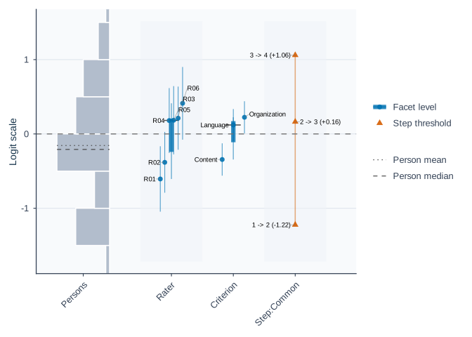
The fit-only summary reports FormalInference = "No"
until precision evidence is supplied. Read the diagnostic decision’s
Why and NextAction together with the precision
checks. A model_based label alone does not override a
failed fit-readiness component or justify a particular substantive
claim.
Infit and Outfit describe departures from the fitted response model; their reference value is 1. A global average near 1 can coexist with local problems. In this example the MML person uncertainty is posterior SD, while the non-person SEs use observed information. Report the basis and interval method when presenting uncertainty; do not call every interval a posterior quantile interval or treat a point difference as a significance test.
3. Identify what needs closer inspection
Are the rating categories working as intended? Examine category use and the transitions between scores on the declared rubric:
scale_toy <- rating_scale_table(fit_toy, diagnostics = diag_toy)
scale_toy$category_table[, c("Category", "Count", "AvgMeasure", "ExpectedMeasure", "Infit", "Outfit")]
#>   Category Count AvgMeasure ExpectedMeasure     Infit    Outfit
#> 1        1    62 -1.1301948      -0.9800341 1.5434694 1.3053867
#> 2        2    96 -0.3122625      -0.3542280 0.4933638 0.5214360
#> 3        3    78  0.3049905       0.2393630 0.3395566 0.3440066
#> 4        4    46  0.8317919       0.7442696 1.9416014 1.8255900
scale_toy$model_context
#>   Model Method StepOwner  StepSelection SlopeOwner            StepScale
#> 1   RSM    MML    Common not_applicable            centered_step_offset
scale_toy$owner_category_table[, c(
  "StepFacet", "CategoryLabel", "RawCount", "Count", "Percent", "UsageStatus"
)]
#>   StepFacet CategoryLabel RawCount Count  Percent UsageStatus
#> 1    Common             1       62    62 21.98582    observed
#> 2    Common             2       96    96 34.04255    observed
#> 3    Common             3       78    78 27.65957    observed
#> 4    Common             4       46    46 16.31206    observed
scale_toy$threshold_table[, c("StepFacet", "Step", "Estimate", "SE", "CIUse")]
#>   StepFacet   Step   Estimate        SE             CIUse
#> 1    Common Step_1 -1.2229852 0.1689986 primary_reporting
#> 2    Common Step_2  0.1634468 0.1670937 primary_reporting
#> 3    Common Step_3  1.0595384 0.1765225 primary_reporting
plot(scale_toy)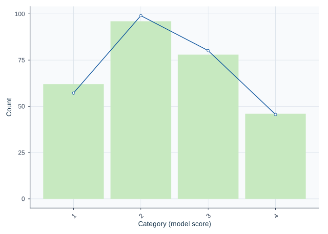
scale_toy$notes
#> [1] "Step owner: Common; selection: not_applicable."
#> [2] "A Step describes the transition between adjacent score categories, not a learning stage or a pass/fail cut. At the corresponding predictor value, the two categories have equal probability, not necessarily probability 0.5 each. Stored step offsets and full ability-axis crossings differ when other facet effects or interactions are included; check the reference profile and step owner."
#> [3] "Category counts are observed ratings, not independent Persons. Owner percentages use each owner's total weight; no-exposure percentages are unavailable."
#> [4] "An unobserved category does not establish structural absence. Review the rating plan and rubric before merging categories."
#> [5] "Step SEs describe the stored step offsets, not full ability-axis crossings, adjacent-step gaps or decision cuts. No additional covariance calculation is requested."
#> [6] "Legacy step uncertainty without full source identity is retained for review; inspect SE_Status, CIUse and UncertaintySourceStatus."
AvgMeasure is the average oriented generating measure
among responses in each observed category; ExpectedMeasure
is its model expectation. Category residual mean squares are descriptive
and have no universal unit baseline.
StepOwner tells you which facet supplies the thresholds.
This RSM has one Common family, so its owner counts
describe the whole sample. With PCM,
step_facet = "Criterion" gives counts and thresholds for
each criterion; step_facet = "Rater" gives them for each
rater. Choose the owner from the rubric and analysis question.
Criterion-owned thresholds cannot describe differences in raters’
threshold spread.
RawCount counts rating rows; Count sums
their weights, and Percent uses the total weight within the
indicated owner level. These are not counts of independent persons. A
category unused by one owner can be common overall.
UsageStatus distinguishes unobserved categories,
zero-weight observations and owners with no ratings; the last have
unavailable percentages. An observed zero does not establish that a
category is structurally impossible.
The threshold table reuses SEs and intervals from the supplied
diagnostics. Check SE_Status, CIUse and
UncertaintySourceStatus before reporting them. Without
diagnostics, the same call returns counts and fitted threshold points
without requesting covariance calculations; its SEs are unavailable.
Notes remain in the returned object, outside the plot.
The bars show observed category counts; the line shows fitted expected counts. Look for rarely used categories, changes in average person measure across categories, and threshold order. Explain the observed pattern in terms of the rubric. A warning is a reason to investigate, not an automatic instruction to merge categories.
Which ratings differ most from model expectations? This example uses an explicit exploratory rule and shows up to ten cases:
unexpected_toy <- unexpected_response_table(
  fit_toy,
  diagnostics = diag_toy,
  abs_z_min = 1.5,
  prob_max = 0.4,
  top_n = 10
)
unexpected_toy$summary
#> # A tibble: 1 × 10
#>   TotalObservations EvaluatedObservations UnavailableObservations UnexpectedN
#>               <int>                 <int>                   <int>       <int>
#> 1               282                   282                       0          21
#> # ℹ 6 more variables: UnexpectedPercent <dbl>, LowProbabilityN <int>,
#> #   LargeResidualN <int>, Rule <chr>, AbsZThreshold <dbl>, ProbThreshold <dbl>
unexpected_toy$table[, c("Person", "Rater", "Criterion", "Observed", "Expected", "StdResidual")]
#>    Person Rater    Criterion Observed Expected StdResidual
#> 1    P016   R02 Organization        4 1.712717    3.204010
#> 2    P012   R03 Organization        4 1.881621    2.769635
#> 3    P048   R06 Organization        4 2.126046    2.291484
#> 4    P021   R04      Content        1 2.867349   -2.214482
#> 5    P025   R04     Language        1 2.815285   -2.139004
#> 6    P003   R01 Organization        1 2.765869   -2.070969
#> 7    P013   R02      Content        2 3.439682   -2.097409
#> 8    P024   R03     Language        4 2.317510    1.993303
#> 9    P024   R03      Content        1 2.656778   -1.931313
#> 10   P018   R02     Language        4 2.340191    1.961204
plot(unexpected_toy)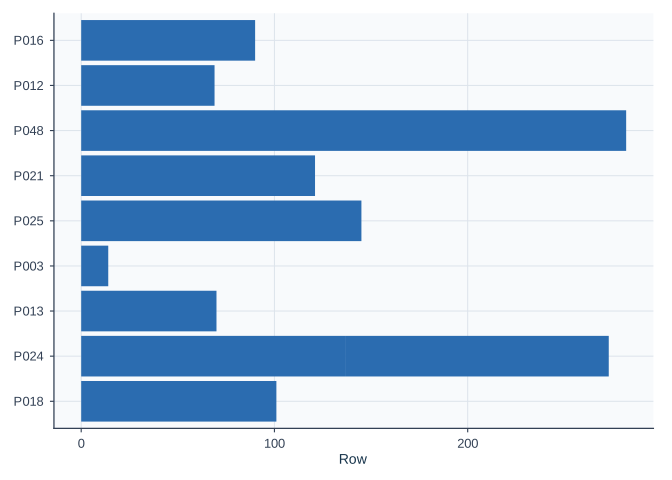
Read the rule in $summary with the residuals. The
displayed cases are a selected preview; top_n limits the
table, while the summary counts all flagged ratings. Here this broad
rule flags 141 of 282 ratings (50%), although only ten cases are
displayed. Report the rule with the count and percentage. Inspect the
original work and scoring context before changing a rating or excluding
a person. A flag does not identify its cause.
The default diagnostics retain the residual/EAP path and the latent-integrated marginal screening path. The latter includes category and pairwise agreement gaps. Keep their bases separate when reporting:
diagnostic_summary_toy$diagnostic_basis[, c("DiagnosticPath", "Status", "ReportingUse")]
#> # A tibble: 4 × 3
#>   DiagnosticPath                   Status        ReportingUse
#>   <chr>                            <chr>         <chr>
#> 1 legacy_residual_fit              computed      legacy_compatibility_screen
#> 2 strict_marginal_fit              computed      screening_only
#> 3 strict_pairwise_local_dependence computed      screening_only
#> 4 posterior_predictive_follow_up   not_available screening_only
plot(fit_toy, type = "marginal_fit", diagnostics = diag_toy)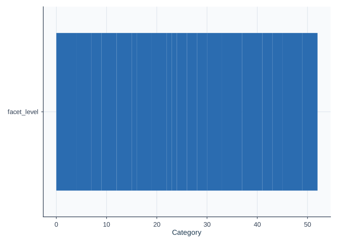
Follow a pairwise warning with plot(). Add residual PCA
only when residual structure is relevant to the question, using
diagnose_mfrm(fit_toy, residual_pca = "both"). Report the
mode and limits of the screen; residual PCA alone does not establish
unidimensionality. See MML
estimation and marginal-fit diagnostics and
vignette("mfrmr-visual-diagnostics", package = "mfrmr") for
these follow-ups.
What should I discuss with a rater? Start from the coverage and category checks above, then view severity and its uncertainty alongside the screening results. Reuse the same fit and diagnostics:
plot(fit_toy, type = "rater_severity", diagnostics = diag_toy, facet = "Rater", show_bands = FALSE)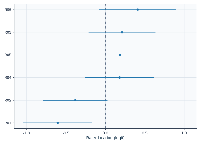
rater_review <- facet_quality_dashboard(
  fit_toy, diagnostics = diag_toy, facet = "Rater"
)
knitr::kable(
  rater_review$detail[, c("Level", "N", "Estimate", "SE", "Infit", "Outfit")],
  digits = 3, row.names = FALSE, caption = "Rater estimates and fit"
)| Level | N | Estimate | SE | Infit | Outfit |
|---|---|---|---|---|---|
| R01 | 47 | -0.606 | 0.224 | 0.772 | 0.757 |
| R02 | 56 | -0.382 | 0.209 | 0.954 | 1.015 |
| R03 | 50 | 0.212 | 0.217 | 1.011 | 0.981 |
| R04 | 47 | 0.180 | 0.223 | 0.917 | 0.891 |
| R05 | 44 | 0.184 | 0.234 | 0.648 | 0.640 |
| R06 | 38 | 0.412 | 0.249 | 0.820 | 0.798 |
knitr::kable(
  rater_review$detail[, c("Level", "MissingMetrics", "SeverityFlag", "MisfitFlag")],
  row.names = FALSE, caption = "Availability and screening flags"
)| Level | MissingMetrics | SeverityFlag | MisfitFlag |
|---|---|---|---|
| R01 | FALSE | FALSE | |
| R02 | FALSE | FALSE | |
| R03 | FALSE | FALSE | |
| R04 | FALSE | FALSE | |
| R05 | FALSE | FALSE | |
| R06 | FALSE | FALSE |
rater_review$settings
#>                                   Setting Value
#> facet                               facet Rater
#> facet_source                 facet_source  user
#> severity_warn               severity_warn     1
#> misfit_warn                   misfit_warn   1.5
#> misfit_lower                 misfit_lower   0.5
#> central_tendency_max central_tendency_max    NA
#> bias_count_warn           bias_count_warn     1
#> bias_abs_t_warn           bias_abs_t_warn     2
#> bias_abs_size_warn     bias_abs_size_warn   0.5
#> bias_p_max                     bias_p_max  0.05
#> bias_source_bundles   bias_source_bundles     0
writeLines(strwrap(rater_review$notes, width = 72))
#> Flags are screening prompts, not evidence of invalid ratings or grounds
#> for automatic exclusion.
#> Severity is relative to the fitted reference; inspect workload,
#> category use and common ratings before comparing levels.
#> FlagCount counts observed flags only. MissingMetrics identifies
#> unavailable diagnostics; zero flags does not mean all checks passed.
#> BiasCount counts flagged cells in supplied bias results only; zero does
#> not establish absence of bias.
#> Stored fit readiness plus numerical, data-support, connectivity, and
#> stability checks passed. Treat this display as diagnostic evidence, not
#> automatic publication approval.
#> Legacy CentralTendencyFlag is disabled by default because origin
#> proximity does not diagnose observed category avoidance or range
#> restriction.
#> No level-level flags were triggered under the current thresholds.
A more severe rater is not necessarily inconsistent or incorrect.
Individual interval overlap is not a test of the difference between two
raters. Read MissingMetrics before interpreting flags: zero
observed flags is not a complete pass when diagnostics are unavailable.
A REVIEW ONLY label retains the fit’s restrictions; the
plot does not override them.
With the unmodified package defaults (absolute severity at least 1
logit, Infit or Outfit at or beyond 0.5 and 1.5), none of the six raters
is flagged in this synthetic example. Session options can change the
misfit band: check rater_review$settings before comparing
your output. A numeric misfit_warn = 1.5 instead selects a
lower bound of about 0.67; it does not preserve the default 0.5. These
bands prompt review, not a verdict on quality. The earlier
response-level screen still selected 141 ratings: the two screens assess
different units and use different rules. Neither result establishes that
every rating is appropriate.
Use the selected unexpected ratings to discuss the rubric and scoring
context, not to automatically exclude a rater. Limited overlap may call
for more shared ratings before comparing raters. A change after training
alone does not establish a training effect. For your own analysis, use
csv_fit and csv_diagnostics, and replace
"Rater" with your actual facet name. Keep the whole
dashboard with saveRDS() to retain its settings and notes;
export_mfrm_bundle(..., include = c("dashboard", "html"))
includes them with the exported tables. See
?facet_quality_dashboard for that export route.
4. Assemble the evidence for a report
res_toy <- mfrm_results(fit_toy, diagnostics = diag_toy, include = "publication")
report_toy <- mfrm_report(res_toy, style = "apa")
report_toy$first_screen[, c("Area", "Status", "MainIssue", "NextAction")]
#>                Area            Status
#> 1           Overall            review
#> 2               Fit            review
#> 3        Bias / DFF request_if_needed
#> 4 Linking / anchors request_if_needed
#> 5  Misfit / pathway request_if_needed
#> 6         Precision                ok
#>                                                                       MainIssue
#> 1 ok=1; review=1; caveat=0; request_if_needed=3; not_computed=0; unavailable=0.
#> 2                  ReviewSignalCount = 9; underfit=0; overfit=0; df_sensitive=9
#> 3                                                   Evidence was not requested.
#> 4                                                   Evidence was not requested.
#> 5                                                   Evidence was not requested.
#> 6                                               No report-index review signals.
#>                                                                 NextAction
#> 1                                                          Start with Fit.
#> 2 Inspect the primary evidence table and template boundary before writing.
#> 3                       Request this evidence only if the claim is needed.
#> 4                       Request this evidence only if the claim is needed.
#> 5                       Request this evidence only if the claim is needed.
#> 6                  Use the listed template route if this area is reported.

checklist_toy <- reporting_checklist(fit_toy, diagnostics = diag_toy)
subset(checklist_toy$checklist, !DraftReady,
       c("Section", "Item", "NextAction"))
#>                        Section                          Item
#> 8               Method Section Hierarchical structure review
#> 10                  Global Fit              PCA of residuals
#> 23 Bias / Interaction Analysis            Facet pairs tested
#> 24 Bias / Interaction Analysis  Screen-positive interactions
#> 27             Visual Displays          Residual PCA visuals
#> 30             Visual Displays       Strict marginal visuals
#> 31             Visual Displays            Bias / DIF visuals
#>                                                                                                                                   NextAction
#> 8  Run `analyze_hierarchical_structure(fit)` once per design and pass the result to `reporting_checklist(..., hierarchical_structure = hs)`.
#> 10                                                                Run residual PCA if you want to comment on unexplained residual structure.
#> 23                                                                   Run bias screening if the manuscript needs interaction-level follow-up.
#> 24                                                                         Run bias screening before discussing interaction-level anomalies.
#> 27                                                     Run residual PCA if you want scree/loadings visuals for residual-structure follow-up.
#> 30             Treat strict marginal plots as exploratory corroboration screens, then corroborate with design review and legacy diagnostics.
#> 31                                                                    Run bias or DIF screening before discussing interaction-level visuals.
DraftReady describes available drafting material with
caveats. An unrequested bias or linking analysis may be irrelevant to
the question; do not run every helper merely to turn every flag
TRUE. The report’s gaps concern the supplied analysis
objects. They cannot confirm recruitment, rater training, ethics, the
study rationale, or whether the prose answers the research question.
For a journal article, the companion
vignette("mfrmr-reporting-and-apa", package = "mfrmr")
provides a Manuscript coverage map: what to report,
where the numerical evidence is, and what the author must supply. It
also shows estimates with uncertainty, reliability and agreement with
distinct interpretations, and a worked question-to-result
explanation.
5. Display a table and save the analysis
measurements_toy <- fit_measures_table(fit_toy, diagnostics = diag_toy)
rater_table_toy <- subset(
  measurements_toy$table, Facet == "Rater",
  c("Level", "N", "Measure", "SE", "CI_Lower", "CI_Upper", "Infit", "Outfit")
)
apa_table(rater_table_toy, digits = 3,
          caption = "Rater severity and fit",
          note = "N counts rating rows. Rater effects are centered within facet and measured in logits; higher values indicate more severe ratings. Intervals are 95% normal approximations from MML observed-information SEs. Infit and Outfit have reference value 1.")
#> Rater severity and fit
#>  Level  N Measure    SE CI_Lower CI_Upper Infit Outfit
#>    R05 44   0.184 0.234   -0.275    0.643 0.648  0.640
#>    R01 47  -0.606 0.224   -1.046   -0.166 0.772  0.757
#>    R06 38   0.412 0.249   -0.077    0.901 0.820  0.798
#>    R04 47   0.180 0.223   -0.256    0.616 0.917  0.891
#>    R02 56  -0.382 0.209   -0.791    0.027 0.954  1.015
#>    R03 50   0.212 0.217   -0.212    0.637 1.011  0.981
#> Note. N counts rating rows. Rater effects are centered within facet and measured in logits; higher values indicate more severe ratings. Intervals are 95% normal approximations from MML observed-information SEs. Infit and Outfit have reference value 1.
Report the score scale and direction with the table. For person results, state the EAP/posterior-SD basis; for rater results, explain that variation in severity is different from inconsistent scoring. Add a sentence answering the study’s question instead of repeating every cell of the table.
# A new temporary directory keeps this synthetic example repeatable
export_dir <- tempfile("mfrmr-workflow-export-")
export_toy <- export_mfrm_results(
  res_toy,
  output_dir = export_dir,
  include = c("default", "report"),
  acknowledge_sensitive = TRUE
)
export_preview <- head(export_toy$written_files[, c("Component", "Format", "Path")])
export_preview$Path <- basename(export_preview$Path)
knitr::kable(export_preview, row.names = FALSE,
caption = "First six exported files (filenames only)")| Component | Format | Path |
|---|---|---|
| summary_overview | csv | mfrmr_results_summary_overview.csv |
| summary_decision | csv | mfrmr_results_summary_decision.csv |
| summary_status | csv | mfrmr_results_summary_status.csv |
| summary_fit_readiness | csv | mfrmr_results_summary_fit_readiness.csv |
| summary_fit_readiness_components | csv | mfrmr_results_summary_fit_readiness_components.csv |
| summary_fit_readiness_parameters | csv | mfrmr_results_summary_fit_readiness_parameters.csv |
This archive retains the collected results.
acknowledge_sensitive = TRUE is used because the example
contains synthetic data; it does not remove identifiers or local paths
from real analyses. Review the files before sharing them. The table
previews six filenames; export_toy$written_files retains
the full list, and its Path column locates the generated
files. Temporary files are for practice; choose a study directory for an
archive you will keep. To reopen the saved analysis without fitting or
computing diagnostics, locate the RDS in that file list:
results_file <- subset(export_toy$written_files, Component == "results_rds")$Path
restored_results <- readRDS(results_file)
summary(restored_results)$decision
#>               Interpretation FormalInference FitReadiness
#> 1 Ready for formal inference             Yes        ready
#>                                                                                                                                                                                                                                 Why
#> 1 All stored fit-readiness components passed. These checks assess numerical readiness and the requested precision method under the specified model; they do not establish model adequacy or finite-sample coverage for this design.
#>                          NextAction
#> 1 Read the compact results summary.
This restores the collected results and diagnostics. The separate
dashboard object rater_review still needs its own
saveRDS() call as described above. The exported replay
script also reloads the complete RDS; it does not need fit
or diagnostics from the original session. Run it with
source("path/to/mfrmr_results_replay.R", chdir = TRUE),
replacing the path with the exported script’s location. Keep your
original data-to-fit script when you also need to reproduce estimation.
For a fit replay including its input CSV, and for saving a manuscript
table, figure, and their notes, follow Section 5 of
vignette("mfrmr-reporting-and-apa", package = "mfrmr").
Further analyses should answer a stated question
For observed rating agreement, start with the rating-agreement tutorial. Its small runnable example shows how to match person-by-task records, distinguish correlation from agreement, compare a score source with a reference, and audit missing pairs without fitting another model. It also explains why these coefficients answer a different question from rater severity or separation reliability.
For prior sensitivity or an external Bayesian extension, use
export_mfrm_model() either with a unit-weight RSM/PCM or
one-family GPCM MML fit, or directly with rating data and a
model spec list when native MML optimization is not needed
first (add write_json = TRUE on Stan bundles to write
CmdStanR-compatible model-data.json alongside
model-data.rds). Both Stan and brms retain supported fixed
facet anchors and group means. This example reuses the RSM fit
above:
# Reuse the fit above; no additional estimation or backend is needed to export.
stan_model <- export_mfrm_model(
  fit_toy, tempfile("stan-model-"), format = "stan",
  acknowledge_sensitive = TRUE
)
brms_model <- export_mfrm_model(
  fit_toy, tempfile("brms-model-"), format = "brms",
  acknowledge_sensitive = TRUE
)
names(stan_model$files)
#> [1] "model-data.rds" "levels.csv"     "categories.csv" "model.stan"
#> [5] "run.R"          "README.txt"     "summarize.R"
model_data <- readRDS(stan_model$files[["model-data.rds"]])
model_data$categories
#>   Category InternalScore Score
#> 1        1             1     1
#> 2        2             2     2
#> 3        3             3     3
#> 4        4             4     4
model_data$priors
#> $ability
#> [1] "independent normal(0, 1)"
#>
#> $location_marginal_sd
#> [1] 1
#>
#> $step_marginal_sd
#> [1] 1
Each directory contains code, data, category/level mappings and
run.R. stan_model$output_dir and
brms_model$output_dir locate these practice bundles;
replace tempfile() with a study directory to retain them.
The category table maps the external model’s integers back to the
original rubric. model_data$levels identifies the Persons
and facet levels, and model_data$step_owners identifies the
shared RSM or facet-specific PCM steps. Set
location_prior_sd and step_prior_sd in
export_mfrm_model() when creating a bundle for a different
prior choice; both formats use those values. Review its README and
priors, then run the script from that directory with CmdStanR/CmdStan
installed (and brms for the second format). Export itself needs neither
backend. Both formats preserve adjacent-category probabilities, the
fixed standard-normal ability scale, facet signs and constraints, and
unordered step offsets with their original sum constraints. Their
explicit structural priors make this a Bayesian analysis; it does not
reproduce MML point estimates or qualify frequentist interval coverage.
Two-family GMFRM also supports Stan export, with explicit component
log-slope priors and a slope-levels.csv mapping; see the two-family
workflow. One-family GPCM uses log_slope_prior_sd in
both formats, with geometric-mean-one slopes. For brms, the source must
use gpcm_mml_identification = "fixed_standard_normal". The
default one-family GPCM estimates the population mean and variance. You
can export its intercept-only population to Stan with
population_prior = list(mean = c(0, 1), log_sd = c(0, 0.5));
each pair gives the location and scale of a normal prior. The mean and
SD are sampled while relative slopes and anchors retain the native
metric. brms still requires the fixed-population specification. Changing
that setting changes the model; do not change it merely to enable
export. Review prior predictions and sensitivity.
Anchor values are exact constraints. levels.csv and
steps.csv in anchored or one-family bundles show the prior
means, marginal SDs and fixed coordinates. A zero SD reflects a fixed
value, not evidence that its earlier calibration was certain. The scope
excludes JML/Person anchors, two-family brms, nonunit weights,
population regression, interactions and shrinkage. Native two-family
fitting still excludes anchors. Inspect sampler diagnostics and prior
sensitivity before using the posterior. Exported ratings and original
labels require the same sharing review as an analysis archive. See
?export_mfrm_model for supported post-processing and
prediction targets.
After sampling, start with summary-decision.csv: it
states the sampling review and next action before presenting estimates.
sampling-review.csv lists the checks and criteria.
parameter-summary.csv keeps original labels, the meaning of
larger values, fixed/estimated status and interval status beside the
numbers. Fixed values have no estimated interval; finite intervals for
estimated values can still require sampling review. Both formats support
Rscript run.R --summarize to rebuild these reports from
saved draws without sampling again. A clean sampling screen does not
establish model validity.
Bring those summaries back into mfrmr with
read_mfrm_posterior(). This small included example has
short chains and intentionally retains a sampling-review status. It
demonstrates the reporting path without fitting or requiring Stan.
posterior <- read_mfrm_posterior(system.file(
  "extdata", "posterior-example", package = "mfrmr"))
summary(posterior)
#> External Bayesian measurement summary
#> GPCM | Stan | Fixed N(0,1)
#> Review sampling before interpreting intervals
#> Why: Fewer than four chains; Chain mixing (R-hat) needs review; Effective sample size for central summaries needs review
#> Next: inspect $checks, then model fit, prior sensitivity and target-specific MCSE.
#> 53 mapped parameters; fixed values have no estimated interval.
#>                Parameter         Role   Mean  Lower  Upper        Interval
#>             Person: p001    estimated -0.403 -1.414  0.543 Sampling review
#>                 Task: t1 fixed_anchor  0.400     NA     NA     Fixed value
#>                 Task: t2    estimated -0.272 -0.471 -0.078 Sampling review
#>  Step owner: r1 | 0 -> 1 fixed_anchor  0.250     NA     NA     Fixed value
#>  Step owner: r1 | 1 -> 2    estimated -1.061 -1.997 -0.058 Sampling review
#>                 Task: t1    estimated  0.635  0.445  0.887 Sampling review
#> Use $parameters, confint(x), plot(x), or mfrm_report(x). Sampling checks do not establish model validity.
posterior_plot <- plot(posterior, quantity = "location", draw = FALSE)
posterior_report <- mfrm_report(posterior, style = "apa")
For your analysis, supply the export directory instead. Use
as_ggplot(posterior_plot) for an editable figure,
plot_data(posterior_plot, "table") for its long table, and
mfrm_report(posterior, output = "html") for the full
report. confint(posterior) retrieves saved 95%
credible intervals, keeping fixed values and review
flags. Other levels, contrasts, predictions and density/raincloud plots
need the backend’s joint draws; they cannot be recovered from this
summary.
| Question | Follow-up |
|---|---|
| How uncertain is a specified difference between two raters? |
mfrm_facet_intervals() uses their covariance; choose
the model-based or sandwich method for the sampling assumptions. Attach
the result with mfrm_results(fit, intervals = ...). See
mfrmr-facet-intervals; an ordinary Wright map does not
switch to sandwich intervals. |
| Do category thresholds need to differ by criterion? |
compare_mfrm() and
mml_quadrature_sensitivity(); fit candidates to the same
observations and review numerical sensitivity. |
| Which facet combinations merit closer review? |
estimate_all_bias(fit) explores all non-Person pairs.
summary(screens)$overview shows availability and magnitude;
$cells preserves signed shifts and counts. Use
plot(screens) and
plot(screens, pair = "Rater x Criterion") for overview and
detail. These conditional screens have no collection-wide multiplicity
control. |
| Do prespecified rater-by-criterion or group contrasts depart from the model? |
estimate_bias() supplies conditional screening
evidence; analyze_dff() has its own scope. For jointly
fitted interactions, see fit_mfrm(facet_interactions = ...)
and interaction_effect_table(). Specify the target,
supported inference route and multiplicity plan before inspecting
results. See the reporting vignette and
mfrmr-linking-and-dff. |
| How often does a declared rater-warning rule detect a specified departure or falsely flag an unaffected rater? |
mfrm_screening_performance() with known simulation
truth and all planned trials. See
mfrmr-screening-performance for individual/family rates,
unavailable results and Monte Carlo uncertainty. |
| Would the conclusions change under a GPCM? |
mfrmr_output_guide("gpcm_capabilities") and
mfrmr-gpcm-scope; explain what discrimination reweighting
means for the score interpretation. |
| Are scores missing from assigned rating events? | Start with the assignment roster, then
review_mfrm_imputations(), fit_mfrm_imputed()
and pool_mfrm_imputed(). See
mfrmr-response-imputation for an explicit imputation model;
the review function does not generate scores. Do not fill unassigned
combinations. |
| Do external attributes describe different groups of persons, raters or tasks? |
mfrm_features() with PCA/k-means for numeric features,
or PAM/hierarchical clustering for mixed features. See
mfrmr-external-features for missing attributes, group
stability and links back to rating events. Groups are not ability
classes or judgments of rater quality. |
| Would more raters or tasks improve observed-score dependability? |
mfrm_g_study() followed by mfrm_d_study();
declare the observed-score design, candidate plans and any composite
weights. Their help explains G/Phi and SEM. These coefficients describe
observed scores, not MFRM latent abilities. |
| Are forms or waves on a comparable scale? |
mfrmr-linking-and-dff and
mfrmr-portable-calibration; common labels alone do not
establish linking. |
| How does a proposed rating design perform under stated assumptions? |
build_mfrm_sim_spec(),
simulate_mfrm_recovery(), and
assess_mfrm_recovery(); report generating conditions,
repetitions, failures, and Monte Carlo uncertainty. |
| How should new persons be scored under an existing calibration? |
predict_mfrm_units() and
sample_mfrm_plausible_values(); reuse an eligible fitted
calibration and report the conditioning assumptions. |
| How certain is a person’s placement relative to supplied ability cuts? | For ordinary RSM/PCM, use cut_scores in the eligible
scoring API and inspect $decisions.
apa_table(..., which = "decisions") retains probabilities,
priors and review states. Check whether the scoring prior represents the
target population; numerical checks do not establish that match. See
mfrmr-portable-calibration for interpretation and
saved-score reporting; calibration and estimated-prior uncertainty are
excluded. |
For repeated simulation work, supply file to
simulate_mfrm_recovery() or
evaluate_mfrm_design(). An identical call reads a finished
result or resumes saved trials after interruption. For example, create a
results directory once and keep this call in the analysis script:
dir.create("results", showWarnings = FALSE)
recovery <- simulate_mfrm_recovery(
  n_person = 50, n_rater = 4, n_criterion = 4,
  reps = 100, seed = 20261021, file = "results/recovery.rds"
)
summary(recovery)$rep_overview  # Retains failed attempts, too.
The default file_refit = "never" rejects a file whose
inputs, fitting controls, replication count, RNG kind or
implementation/software identity differ. Use a new path to preserve both
studies, or explicitly choose "on_change" to replace an
incompatible study. "always" starts again even if the file
matches. After completion, ordinary readRDS() also loads
the result and its reproducibility metadata. Save the
script and software environment with it; seed recording is not a
guarantee of identical numerical results on every platform. See
?simulate_mfrm_recovery for checkpoint boundaries and
parallel resumption.
For an injected Group-by-Criterion or Rater-by-Criterion departure,
evaluate_mfrm_signal_detection() summarizes the behavior of
the selected screen. Start with
summary(x)$detection_summary: compare the planned and
available counts before interpreting a rate. Non-target rates average
the available-cell proportion within each contributing trial; they are
neither pooled-cell rates nor the probability of any false flag. Inspect
x$rep_overview for failed stages and seeds, and
x$results for target-level unavailability reasons. This
helper uses saveRDS() for saving the returned result,
without the checkpoint arguments shown above.
DIF contrasts are reference minus focal. A residual-score difference
is not the injected latent effect; a subgroup location difference
requires common-scale linking before its mean is reported. The bias
shift is relative to the fitted baseline. These summaries do not
establish effect recovery or calibrated power. Residual DIF tests remain
unavailable, and refit/bias rates remain screening summaries. See
?evaluate_mfrm_signal_detection for denominators, Monte
Carlo uncertainty and interpretation of older saved results.
When starting from extract_mfrm_sim_spec(fit), inspect
the proposed generating mechanism. Without a population regression, the
Person spread is the SD of the reported estimates; shrinkage and
measurement error mean it need not equal the latent population SD. With
a population regression, the stored coefficients, residual variance,
transformations and factor coding define Person generation. The
generating parameters remain fixed across replications. Monte Carlo SEs
measure the precision of the simulation averages under those
assumptions; they do not measure uncertainty in the original fit or
validate future forecasts. When covariates and observed assignments
belong to the same template Persons, use
population_assignment = "matched" (the default for newly
built/extracted specifications). Matching TemplatePerson
IDs preserve the association between covariates, groups and assignment
patterns. Choose "independent" only when breaking that
association is part of the intended scenario. A population
Group column also defines the response group; conflicting
group definitions are rejected. Truth metadata retain the selected
source template IDs.
Observed skeletons preserve repeated rows and weights. Each row
generates a new conditionally independent rating; dependence across
occasions or among peer reviewers requires a different generating model.
Remove accidental source duplicates before building the specification.
Weights affect fitting and do not create extra generated responses.
Older saved specifications without population_assignment
keep independent template draws; rebuild them and use a new study file
for matched sampling.
For a manual refit of generated latent-regression data, take both
person_data and population_formula from
attr(simulated_data, "mfrm_population_data"). The
formula-compatible terms object retains the template’s transformation
basis and factor coding. Rewriting it as a fresh ~ scale(X)
formula would relearn the scaling on the new cohort. Old transformed
specifications without the stored basis must be rebuilt from the
original template or fit and saved as a new study.
Read recovery results as relative parameter recovery under the
declared generating conditions.
summary(recovery)$recovery_summary reports RMSE and its
Monte Carlo SE across independent trials. Mean-aligned group bias is
zero by construction, so a small value does not establish unbiased
estimation of each parameter. PCM/GPCM comparisons account for the facet
shift induced by centering the generating step thresholds.
For interval evidence, read Coverage95 together with
ExpectedRows, CoverageRows,
CoverageAvailabilityRate, McseCoverage95 and
FailedReps. Coverage is conditional on obtaining a valid
interval; failures and unavailable intervals remain visible separately.
Non-Person MML facet coverage uses each level’s deviation from its facet
mean with the matching covariance. JML point recovery and Person scores
remain useful, but their source uncertainty is not treated as that
structural interval; inspect CIReason in
recovery$recovery or CIReasons in the summary.
Unknown target rosters produce NA rates, not zero or
successful outcomes.
assess_mfrm_recovery(recovery)$uncertainty_review keeps
these counts and reasons with its checklist.
For older saved objects, summary(), assessment and
summary/coverage plotting recalculate the aggregates without fitting.
They withhold legacy coverage when the required covariance was not
saved. A new run is needed for corrected PCM/population truth mapping
and matching interval evidence; retain the old file as a separate study.
The help page explains which fields can be recovered.
For stability against an observed-data reference, use
build_mfrm_resampling_spec() and
draw_mfrm_resamples(). They resample entire Person clusters
within optional strata, retaining all ratings for each selected Person.
A same-size bootstrap requires
design = "stratified_bootstrap",
sample_fraction = 1, and
topup_preserve_facets = FALSE; the default fraction is one
half. Adding Persons to restore missing facet levels changes the
sampling distribution. Read sampling_scheme and the
base/added/final counts in the manifests. Person resampling holds the
observed non-Person facets fixed; it does not reproduce sampling new
raters/tasks or dependence among Persons in a peer-review network.
Full-data estimates are uncertain references, not known truth, and these
helpers do not qualify bootstrap confidence intervals.
Missing attributes and missing rating
scores need different models and workflows. Neither clustering
nor response-score imputation is a prerequisite for ordinary MFRM
analysis. G/D-studies start from observed scores and their design; do
not substitute MFRM estimates or testlet variances for their input. For
these branches, mfrmr_output_guide("features"),
mfrmr_output_guide("imputation") and
mfrmr_output_guide("gtheory") identify the supported
summaries and plots. Save their full objects with
saveRDS(); they have dedicated output routes and are not
mfrm_results() inputs.
Simulation examples with one or two repetitions test the computational setup; they do not estimate operating characteristics adequately for a paper. A simulation’s assumptions and results also do not replace evidence from the observed assessment. Keep these analyses in the report only when their role in answering the study question is clear.
An observed writing-assessment example
The optional sirt package supplies
data.ratings1, observed German-writing ratings from a 2009
Austrian educational standards survey. Its 274 rows contain 135
students, seven observed raters and five rubric criteria scored 0 to 3.
The data
documentation describes the source. This dataset is separate from
mfrmr’s synthetic examples.
The practical question is which differences in severity, category use or consistency merit discussion with a rater. The example below uses a PCM so criteria can have different category thresholds. It assumes a common writing scale and conditionally independent ratings; inspecting the output does not establish those assumptions. Repeated rubric ratings of one performance may still share influences that this model does not represent.
Run this optional example after installing sirt. It is
not run when building this vignette. Display aliases replace source
identifiers in the example’s tables; aliases do not make a rating
archive anonymous.
library(mfrmr)
data("data.ratings1", package = "sirt")
wide <- data.ratings1
persons <- match(wide$idstud, unique(wide$idstud))
raters <- match(wide$rater, unique(wide$rater))
writing <- do.call(rbind, lapply(paste0("k", 1:5), function(criterion) {
  data.frame(
    Person = sprintf("P%03d", persons), Rater = paste0("R", raters),
    Criterion = criterion, Score = wide[[criterion]]
  )
}))
review <- describe_mfrm_data(
  writing, person = "Person", facets = c("Rater", "Criterion"), score = "Score",
  rating_min = 0, rating_max = 3
)
review$row_retention
review$design_connectivity

writing_fit <- fit_mfrm(
  writing, "Person", c("Rater", "Criterion"), "Score",
  method = "MML", model = "PCM", step_facet = "Criterion",
  rating_min = 0, rating_max = 3, quad_points = 61, maxit = 400
)
writing_diagnostics <- diagnose_mfrm(writing_fit, residual_pca = "none")
feedback <- facet_quality_dashboard(
  writing_fit, diagnostics = writing_diagnostics, facet = "Rater"
)
feedback$detail[, c("Level", "N", "Estimate", "SE", "Infit", "Outfit", "MisfitFlag")]
feedback$settings
plot(writing_fit, type = "rater_severity", diagnostics = writing_diagnostics, facet = "Rater", show_bands = FALSE)
saveRDS(feedback, "writing-feedback.rds")
archive <- export_mfrm_bundle(
  writing_fit, diagnostics = writing_diagnostics, facet = "Rater",
  output_dir = "writing-analysis", data = writing, acknowledge_sensitive = TRUE
)
Reshaping gives 1,370 criterion ratings; the 274 original rows are not the number of students. Each rater has 185 to 205 criterion ratings here. The example produces a low-Infit flag for R7: unusually predictable ratings also trigger this screen. This is a prompt to inspect rubric use and individual ratings, not evidence that R7 is inaccurate or should be removed. Severity and consistency answer different questions, and this dataset supplies no known true rater quality against which to validate either interpretation.
The quadrature setting belongs to this example; use
mml_quadrature_sensitivity() when numerical sensitivity
matters to a comparison. Preserve the dashboard’s notes, review
rating-category use and common-person coverage, and use the actual
scripts or rubric descriptors in feedback discussions. A
different-looking result alone does not establish that a rater needs
training or that training would improve the scores.