Compare fit-screening thresholds against known simulation truth

See how detection and false-flag rates change when you change fit-screening thresholds in a simulation with known truth. Apply specified mean-square bands to saved Infit/Outfit values without refitting models. Keep underfit, overfit and their union separate. Here sensitivity analysis means comparing thresholds; the reported Sensitivity rate means detecting an affected target.

Usage

mfrm_screening_sensitivity(
  roster,
  measures,
  thresholds,
  rule,
  statistic = c("either", "infit", "outfit"),
  zstd_cut = NULL,
  level = 0.95
)

# S3 method for class 'mfrm_screening_sensitivity'
summary(object, ...)

# S3 method for class 'mfrm_screening_sensitivity'
print(x, ...)

# S3 method for class 'mfrm_screening_sensitivity'
plot(
  x,
  style = c("tiles", "curves"),
  direction = "either",
  metric = c("false_flags", "detection"),
  condition = NULL,
  quantity = c("rate", "unavailable"),
  draw = TRUE,
  palette = c("accessible", "mono"),
  title = NULL,
  caption = NULL,
  show_title = FALSE,
  show_notes = FALSE,
  show_labels = TRUE,
  text_scale = 1,
  point_size = 2.5,
  ...
)

Arguments

roster

Data frame with Condition, Replicate, Target identifiers and logical Affected: TRUE denotes the prespecified departure that the screen is intended to detect. Include every planned target and replication, including failed runs. Within a condition, use the same targets and truth labels in every replication. Put different designs or methods in separate conditions. Identifiers are matched exactly as character labels.

measures

Data frame with Condition, Replicate, Target, Infit and Outfit. Include InfitZSTD and OutfitZSTD when requesting the combined ZSTD rule. The selected statistic's columns are required; nonfinite values and omitted rows remain unavailable. Additional source columns, such as numerical readiness, are retained without filtering.

thresholds

Data frame with unique nonempty Profile labels and numeric Lower, Upper bounds satisfying 0 < Lower < Upper. Profiles are compared in supplied order, without selecting an optimum.

rule

Nonempty description of the prespecified screen, including its thresholds, comparison family and any selection/refitting procedure.

statistic

"either" (default) flags Infit OR Outfit; "infit" or "outfit" uses only the specified index.

zstd_cut

NULL (default) uses only mean squares. A positive finite number adds directional ZSTD flags with inclusive boundaries. This is an explicit alternative rule, not a significance calibration. Record the chosen df convention and residual definition in rule.

level

Confidence level for exact binomial Monte Carlo intervals; default 0.95. These describe simulation uncertainty, not an interval for rater severity or a guarantee of screening accuracy.

object

An mfrm_screening_sensitivity object.

...

For summary.mfrm_screening_sensitivity(): Unused by print and summary.

For plot(): Unused.

x

Output from mfrm_screening_sensitivity().

Also for summary(): An mfrm_screening_sensitivity object.

style

"tiles" shows a labelled rate matrix. "curves" shows profile comparisons with pointwise Monte Carlo intervals by condition.

direction

One or more of "either", "underfit", "overfit".

metric

"false_flags" or "detection" chooses the family event.

condition

Optional condition labels to display.

quantity

"rate" (default) or "unavailable", the proportion of planned family events whose outcome is unresolved.

draw

For plot(): FALSE returns plot data without opening a device.

palette

"accessible" uses a sequential blue scale for tiles and blue/orange/purple lines with different symbols. "mono" uses greys.

title, caption

NULL uses the default text; a string replaces it; "" removes it. Interpretation notes remain in the saved plot data.

show_title, show_notes

Show the title and caption, respectively. FALSE hides text without deleting its metadata.

show_labels

Show percentages and known/planned counts in tiles.

text_scale

Positive multiplier for text size.

point_size

Positive point size in ggplot millimetres; base graphics use the corresponding relative size (2.5 is the default).

Value

An mfrm_screening_sensitivity object with by_target, by_family, aligned outcomes, replication-level family_outcomes, source roster and measures, thresholds and settings. Each result table identifies Profile, Lower, Upper and Direction; the remaining columns have the meanings documented by mfrm_screening_performance().

For plot(): Invisibly, a ggplot object carrying exact selected tables, settings, notes, and alternative text accessible via plot_data().

Details

Mean-square boundaries are strict: equality is inside the band. Missing values use three-valued logic: TRUE OR NA is TRUE, but FALSE OR NA is NA. The family event counts any affected or any unaffected target once per independent replication. Correlated raters are not independent trials. The source roster fixes truth and planned denominators for every profile. Affected denotes the departure of interest; when comparing directional screens, an affected-target flag can have the wrong direction for that departure. Inspect directions together, not just the union's sensitivity.

Thresholds are review heuristics, not universal error-controlled tests. A low mean square describes low residual variability, not poor rater quality or proof of misconduct. ZSTD is sensitive to sample size and its df convention. Selecting a threshold on these results and reporting its same- sample performance is optimistic; use a separately designed validation. Pointwise Monte Carlo intervals are not simultaneous across profiles or conditions. Their overlap is not a paired test of rules applied to the same replications. No automatic exclusion or refitting is performed.

This helper does not qualify the supplied statistics. In particular, ordinary Rasch bands must not be transferred to extended-model posterior- predictive residual summaries that lack the same reference distribution.

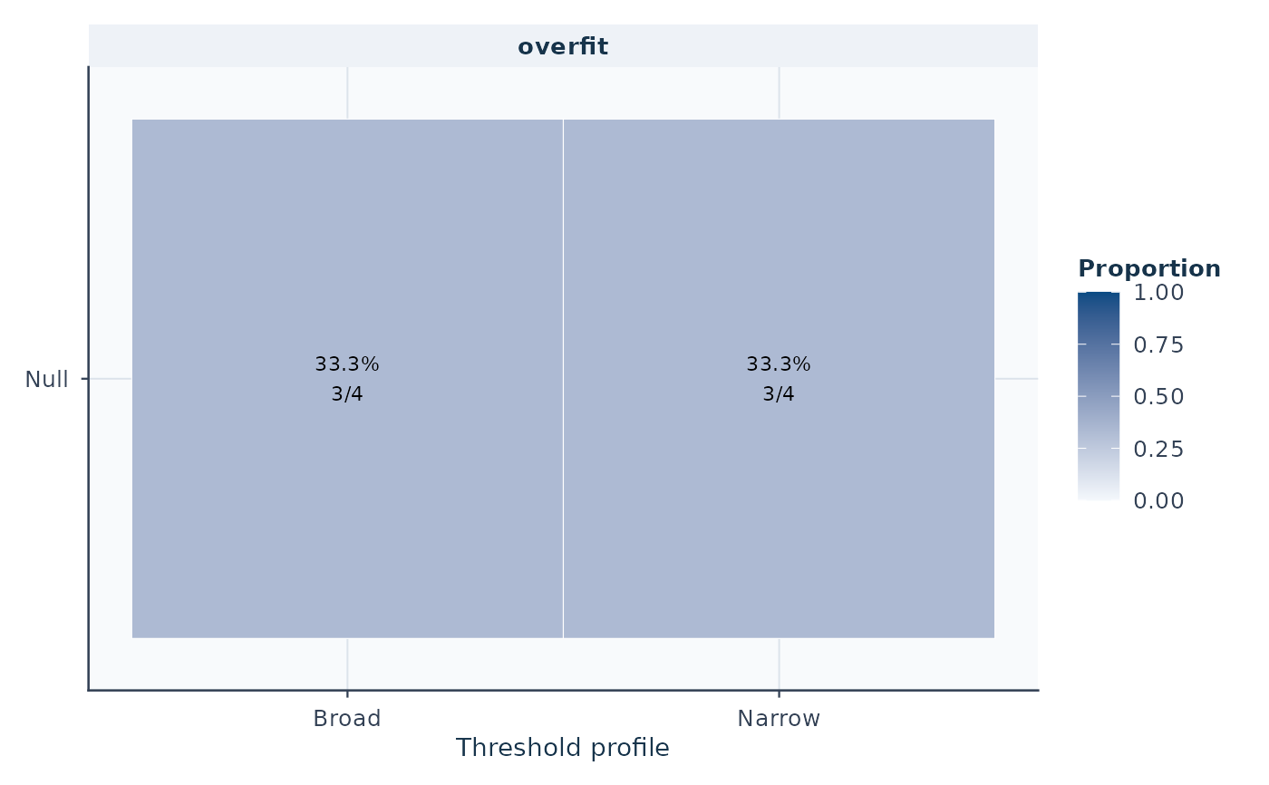
plot() method: Plot directional screening rates across threshold profiles

For plot(): Tile shading is supplemented by numeric labels; missing estimates are labelled NA. Profile order is supplied order, not an optimized ranking. Curves connect discrete profile choices, not a continuous threshold scale. Tile plots do not display uncertainty intervals: consult the retained table or curve view. Exact intervals are pointwise and conditional on known outcomes; all-trial bounds are retained, not confidence intervals.

References

Linacre, J. M. (2003). Size vs. significance: standardized chi-square fit statistic. Rasch Measurement Transactions, 17(1), 918. https://www.rasch.org/rmt/rmt171n.htm.

Examples

roster <- expand.grid(Condition = "Null", Replicate = 1:4,
                      Target = c("R1", "R2"), stringsAsFactors = FALSE)
roster$Affected <- FALSE
measures <- roster[c("Condition", "Replicate", "Target")]
measures$Infit <- c(.45, .8, 1.1, NA, .9, 1.4, 1.2, NA)
measures$Outfit <- measures$Infit
bands <- data.frame(Profile = c("Broad", "Narrow"),
                    Lower = c(.5, .7), Upper = c(1.5, 1.3))
sensitivity <- mfrm_screening_sensitivity(roster, measures, bands,
  rule = "Illustrative fixed-rater residual screen; no exclusion/refit")
plot(sensitivity, direction = "overfit")