Plot fitted MFRM results with ggplot2

Usage

# S3 method for class 'mfrm_fit'
plot(
  x,
  type = NULL,
  facet = NULL,
  top_n = 30,
  theta_range = c(-6, 6),
  theta_points = 241,
  title = NULL,
  palette = NULL,
  label_angle = 45,
  show_ci = NULL,
  ci_level = 0.95,
  group = NULL,
  diagnostics = NULL,
  include_fit_measures = TRUE,
  fit_stat = c("Infit", "Outfit"),
  fit_scale = c("mnsq", "zstd"),
  zstd_method = c("facets", "engine"),
  include_person = FALSE,
  person_subset = NULL,
  top_n_person = 30,
  person_labels = c("flagged", "all", "none"),
  facet_labels = c("all", "flagged", "none"),
  panel = c("combined", "facet"),
  fit_range = c(0.5, 1.5),
  zstd_cut = 2,
  draw = TRUE,
  preset = c("standard", "publication", "compact", "monochrome"),
  renderer = NULL,
  wright_style = c("native", "facets_style"),
  category_labels = NULL,
  rows_per_logit = 2L,
  wright_range = NULL,
  extreme_placement = c("ends", "estimate"),
  persons_per_star = NULL,
  show_title = FALSE,
  show_notes = FALSE,
  marginal = c("auto", "histogram", "none"),
  ...,
  level = NULL,
  view = NULL,
  metric = NULL,
  comparison = NULL,
  labels = NULL,
  highlight = NULL
)

Arguments

x: An mfrm_fit object from fit_mfrm().
type: Plot type. Omit type (or use NULL / "wright") for the primary native Wright map. Use "bundle", "all", or "default" for the three-part fit bundle; otherwise choose one of "facet", "person", "step", "wright", "pathway", "fit_pathway", "ccc", "ccc_surface", or "category_surface". "pathway" is the theta-to-expected-score display; "fit_pathway" is the fit-statistic-to-measure display. Additional diagnostic and reporting views are listed under "Single-fit views" in mfrmr_plot_migration, with replacements for all former helpers.
facet: Optional facet name for type = "facet".
top_n: Maximum number of non-person facet locations retained by the native Wright map for compact displays. Step transitions are always retained separately and do not consume this limit; any omitted facet locations are counted in the returned retention table and disclosed in the plot subtitle/note. Use Inf for a complete all-level final map. The FACETS-style payload always retains every fitted facet and step location.
theta_range: Numeric length-2 range for pathway, CCC, and category-surface plot data.
theta_points: Number of theta grid points used for pathway, CCC, and category-surface plot data.
title: Optional custom title.
palette: Optional color overrides.
label_angle: Rotation angle for x-axis labels where applicable. Native Wright maps reserve bottom space for full labels when abbreviating them would make different groups indistinguishable.
show_ci: Whether to add approximate confidence intervals when available. NULL selects the display-specific default: TRUE for the primary native Wright map and type = "fit_pathway", and FALSE for the FACETS-style ruler and other plot types. With renderer = "facets", explicitly setting show_ci = TRUE creates a hybrid display: FACETS-style ruler grammar with mfrmr uncertainty intervals.
ci_level: Confidence level used when show_ci = TRUE.
group: Optional grouping for type = "wright" to overlay per-group person-density curves (DIF / DFF screening view). Either a column name (looked up first in group_data when supplied through ..., then in fit$prep$data) or a vector aligned with fit$facets$person. Ignored for other type values and for wright_style = "facets_style", whose person column is a single FACETS-style star frequency. To pass the source data alongside, use plot(fit, type = "wright", group = "MyCol", group_data = <df>).
diagnostics: Optional matching output from diagnose_mfrm(). Recompute it after refitting; mismatched or outdated readiness records are rejected. When supplied, Wright-map standard errors and precision metadata reuse matching rows from diagnostics$measures without replacing fitted coordinates, while pathway plot data reuse fit_measures, fit_status, and curve_fit_status instead of recomputing diagnostics. Must match this fitted analysis; see mfrmr_compatibility_layer for migration of saved diagnostics.
include_fit_measures: If TRUE (default), pathway plot data include tidy fit-measure and fit-status tables for custom R graphics. Set to FALSE when only the curve coordinates are needed.
fit_stat: For type = "fit_pathway", the horizontal fit statistic: "Infit" (default) or "Outfit".
fit_scale: For type = "fit_pathway", use mean squares ("mnsq") or standardized fit ("zstd") on the horizontal axis.
zstd_method: For a ZSTD fit pathway, "facets" (default) uses the FACETS/Wright-Masters fourth-moment df, matching diagnose_mfrm(). "engine" retains the former package-native df convention. Neither establishes complete FACETS output equivalence. Refreshing companions from supplied diagnostics preserves their recorded WHEXACT choice.
include_person: If TRUE, include person rows in a fit pathway.
person_subset: Optional character vector of person IDs retained in a fit pathway before ranking.
top_n_person: Maximum person rows retained in a fit pathway, ranked by distance from expected fit. Use Inf for all selected persons.
person_labels: Person-label policy for a fit pathway: "flagged" (default), "all", or "none".
facet_labels: Facet-level label policy for a fit pathway: "all" (default), "flagged", or "none". This changes drawn labels only; all retained facet rows remain in the draw-free table.
panel: Fit-pathway layout: "combined" (distinguish persons by shape) or "facet" (one base-graphics panel per facet).
fit_range: Mean-square review lines for a fit pathway.
zstd_cut: Absolute ZSTD review line for a fit pathway.
draw: If TRUE, print the resulting ggplot object.
preset: Visual preset ("standard", "publication", "compact", or "monochrome").
renderer: Wright-map renderer. Use "native" (default) or "facets" for the FACETS Table 6-style visual layout. This is the canonical selector for new code. The native map is the primary display and includes available facet uncertainty by default. The closest FACETS-style visual uses show_ci = FALSE.
wright_style: Wright-map renderer. "native" preserves the package's histogram, point, range, and facet-SE display. "facets_style" adds a FACETS Table 6-style text ruler with person-frequency stars, signed facet headers, and labeled score-transition lines. It is a visual-layout option, not a claim of numerical equivalence with FACETS. This explicit style name is equivalent to renderer = "facets". Adding show_ci = TRUE to that style is an mfrmr/FACETS hybrid rather than the closest FACETS-style view.
category_labels: Optional score rubric labels used by wright_style = "facets_style". Supply a named character vector keyed by original score, an unnamed vector with one label per retained category, or a data frame with Score and Label columns.
rows_per_logit: Number of FACETS-style ruler rows per logit.
wright_range: Optional finite increasing length-2 logit range for the FACETS-style ruler. NULL derives a range that contains the fitted data.
extreme_placement: In the FACETS-style renderer, place extreme-score persons at the ruler "ends" or retain their fitted "estimate".
persons_per_star: Number of persons represented by one * in the FACETS-style frequency column. NULL chooses a compact value automatically.
show_title: Logical; display the main plot title (default FALSE). Structural panel headings, axis labels, legends, and data labels remain visible.
show_notes: Logical; display explanatory subtitles, footnotes, and review-only title markers. Notes remain available in the returned object, and R warnings are still issued. Default FALSE; use plot_data(p, "notes") for the descriptions and cautions outside the figure.
marginal: Marginal histogram display for two-continuous-variable scatterplots ("auto", "histogram", or "none"). Default "auto" attaches aligned X/Y marginal histograms on single-panel scatterplots with at least 8 finite plotted coordinate pairs.
...: View-specific controls listed in mfrmr_plot_migration. The consolidated routes reject irrelevant or duplicated arguments.
level: Named alternative to ci_level, a single number strictly between 0 and 1. Supply only one of these names, even when equal. Both omitted retain 0.95. This controls the fitted-model plot intervals; attached interval results retain the level chosen when they were computed.
view: Optional display variant for consolidated routes: for example, "pairs" or "heatmap" for agreement, "unified" for the former unified Wright helper, or "funnel" for shrinkage. See mfrmr_plot_migration.
metric: Quantity for a consolidated route, for example "reliability", "separation" or "strata", or "exact" / "correlation" for agreement.
comparison: Another fitted model for paired Wright/CCC displays, or an ordered list of additional fits for type = "trajectory". Plotting does not equate their scales or perform a model-selection test.
labels: Labels for paired models or all trajectory waves, reference first.
highlight: Optional named list of non-person facet level IDs, for example list(Rater = c("R01", "R02")), for Wright maps only (including view = "unified" and the Wright component of a bundle). Selected labels receive a > prefix in both renderers and saved ggplot conversion. Levels outside the usual top_n selection are added, so the displayed count may exceed that limit. Fitted locations and uncertainty do not change; the automatic scale uses all fitted locations before compaction. Selection is not a statistical flag. Inspect locations$Highlighted, retention and notes in the returned plot data. Unknown IDs or levels without finite locations are rejected. NULL selects no levels.

Value

Invisibly, a ggplot object (including a 3-panel composite ggplot when type = "bundle" / "all" / "default"). Each returned fit plot carries its underlying plot payload and notes accessible via plot_data() and plot_data_components(), including domain-specific readiness, an interpretation status, a notes table, display settings, and a one-row scale_contract table recording the fitted coordinate basis, population SD when applicable, discrimination basis, and GPCM MML identification convention.

Details

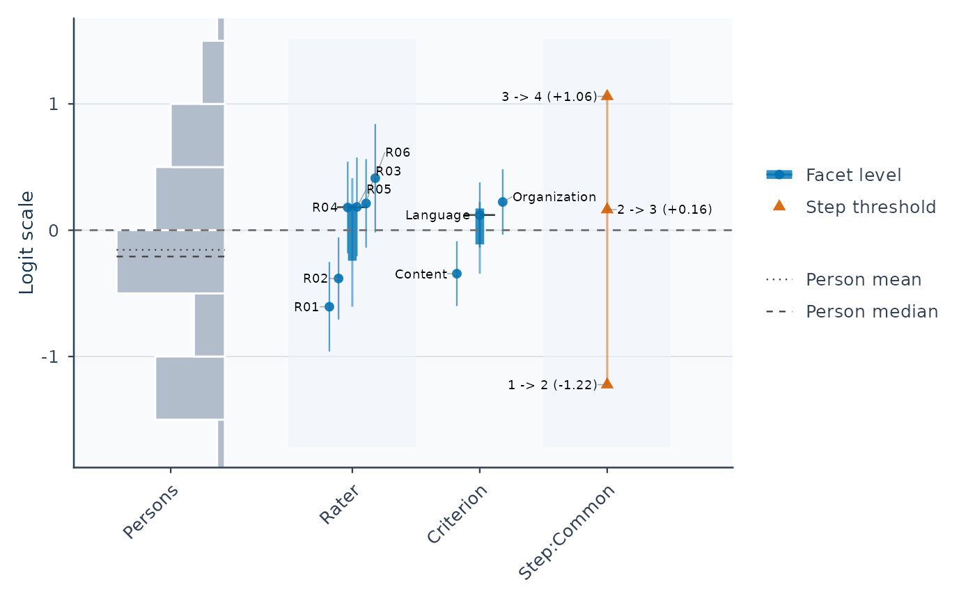
Start with plot(fit): it draws a Wright map of person abilities, rater severities, other facet locations, and category thresholds on one logit scale. No plot options are needed for this first view.

For adjusted-score comparisons, use plot(fit, type = "fair_average", show_ci = TRUE). metric = "FairM" uses mean reference measures; metric = "FairZ" uses a zero reference, not a z-score. PCM averages expectations over administered scales with the table's observation weights and totalscore selection. Its conditional delta-method intervals use the same retained observations as the table: finite direct anchors in ordinary additive RSM/PCM JML are retained even with all-minimum/all-maximum responses, including when totalscore = FALSE. The intervals use the derivative of that same average. RSM/PCM intervals hold thresholds, other effects and reference means fixed; they are diagnostic approximations, not full calibration-uncertainty intervals. Inspect the returned data and notes for the interval method and unavailable rows. See fair_average_table() for reference definitions and plot_fair_average for view-specific controls. For ordinary additive RSM/PCM JML, xtreme = .3, xtreme_method = "facets" requests conditional total-score extrapolation of extreme measures and their fair scores. Primary estimates and fixed anchors are retained. Group-mean anchors are unsupported. The measure SE describes the corrected total; fair-score intervals remain unavailable for positive xtreme. The default xtreme_method = "display" retains the old average-score display convention and leaves fair scores unchanged.

This S3 plotting method provides the core fit-family visuals for mfrmr. When type is omitted, it returns the Wright map alone as a ggplot object (the most useful single figure for a first inspection). Pass type = "bundle" (or "all" / "default") to obtain a three-panel composite ggplot containing a Wright map, pathway map, and category characteristic curves. The compact native default records any omitted facet locations in plot_data(p, "retention") and the returned notes; use top_n = Inf to retain every fitted location in the final Wright map. LabelX / LabelY provide text positions, and leader lines connect displaced labels to unchanged fitted points. Display labels may be shortened; plot_data(p, "label_points") retains the full labels, fitted coordinates and text positions for custom graphics. Step transitions share one vertical ladder and their labels include the fitted threshold logit. When the fit records boundary-separated facet levels and no display range was supplied, the native and FACETS-style maps use the same robust automatic range and place those levels at ruler ends. Exact fitted values and intervals remain in OriginalEstimate, CI_Lower, and CI_Upper; DisplayEstimate, DisplayCI_Lower, DisplayCI_Upper, and the clipping-status columns describe only the rendered coordinates. Endpoint triangles and the returned notes disclose omitted or clipped intervals. The returned object always carries machine-readable metadata accessible through plot_data(), even when the plot is drawn immediately. Titles and explanatory notes are omitted from the figure by default; use show_title = TRUE or show_notes = TRUE to include them. The returned plot_data(p, "notes") table contains Type and Text columns for interpretation, reference-profile conditions, and display/retention notes where applicable; plot_data(p, "display") records the two flags. Original titles, subtitles, coordinates, and readiness metadata are retained. as_ggplot() respects these flags and retains the notes in attr(plot, "mfrmr_notes").

Fit-family Wright, pathway, and CCC displays use a shared, CUD-informed palette. The first eight series use an Okabe-Ito foundation with bright yellow omitted and darker pink/amber/cyan entries for light backgrounds. Beyond eight series, colours come from the dark half of the viridis HCL palette. Expected-score and category curves also vary line type; Wright locations retain their distinct point shapes, and small data labels use dark neutral text. Six line types cycle for larger series sets, so dense plots still require labels, panels, or more space. This is not a guarantee of perceptual separation for every viewer or device. preset = "monochrome" applies to these series. Custom palette values are retained in the plot payload and used during saved-plot conversion; colour overrides keep the non-colour encodings. See https://jfly.uni-koeln.de/color/ for Color Universal Design guidance.

Every fit-derived payload also carries data$fit_readiness, data$interpretation_status, and data$interpretation_note. Availability and interpretability are separate: when a numerical, data, design, or stability status requires review, the coordinates remain available for diagnosis, but the call warns and records the review-only interpretation in the returned metadata. Hiding an annotation changes presentation only; it does not change the fit's interpretation status or suppress warnings. A prior-regularized extreme MML EAP remains in fit$facets$person. If its source fit is blocked, however, it is omitted from the Wright-map scale so that a finite but non-interpretable trace cannot collapse the display. The exact excluded rows and reason remain in data$person_exclusions, and the omission is stated in data$retention_note.

type = "unexpected" uses the same default as unexpected_response_table(): abs_z_min = 3, rule = "residual". The optional rule = "either" or "both" also uses prob_max. Saved table plots retain the recorded thresholds. A fully evaluated screen with no flags yields an empty display and retains its screening summary.

type = "wright" shows persons, facet levels, and step thresholds on a shared logit scale. Estimates are plotted as fitted, so the sign convention follows the fit: higher Person values predict higher coded scores in these positive-discrimination models. Whether that means more comprehensible or less comprehensible speech depends on the rubric coding. Under the default negative orientation, higher non-Person facet values reduce expected coded scores; calling this greater severity/difficulty presumes that higher scores represent better performance. Facets listed in fit_mfrm(positive_facets = ...) are reversed (higher values raise expected scores); state the active orientation in figure captions when reporting. The returned notes, accessible through plot_data(), state the recorded facet directions and the score-coding caveat. Missing orientation in an older or imported result is not guessed. Category labels do not recode the data. See mfrmr_visual_diagnostics for reverse-coded comprehensibility, fit, conditional bias and Step explanations.

Set renderer = "facets" (equivalently, wright_style = "facets_style") for a line-printer-inspired common ruler. That mode retains every facet location in its data and shows actual (original, when scores were internally recoded) adjacent score transitions. Its facets_style payload contains tidy ruler, person-frequency, facet, step, mean-half-score, header, category-label, and settings tables for custom graphics. RulerValue records the nearest discrete ruler row for line-printer reconstruction, whereas step and midpoint lines are drawn at their exact fitted DrawValue and step labels print that logit value. The styling emulates the semantics of FACETS Table 6; estimates and standard errors remain those produced by mfrmr. Use show_ci = FALSE for the closest FACETS-style rendering. If show_ci = TRUE is requested, interpret the result as a hybrid that adds mfrmr uncertainty intervals to FACETS-style ruler grammar. Column headings are retained even on narrow devices. If headings or person frequency stars need more space, drawing warns; use a wider device or increase persons_per_star for a more compact frequency column.

type = "pathway" shows expected score traces and dominant-category regions across theta. This expected-score display is distinct from the Bond-and-Fox-style fit-versus-measure pathway: use type = "fit_pathway" for Infit/Outfit on the horizontal axis and measure logits on the vertical axis. Its draw-free plot data include person-selection settings, CI columns, and explicit SE-source metadata. 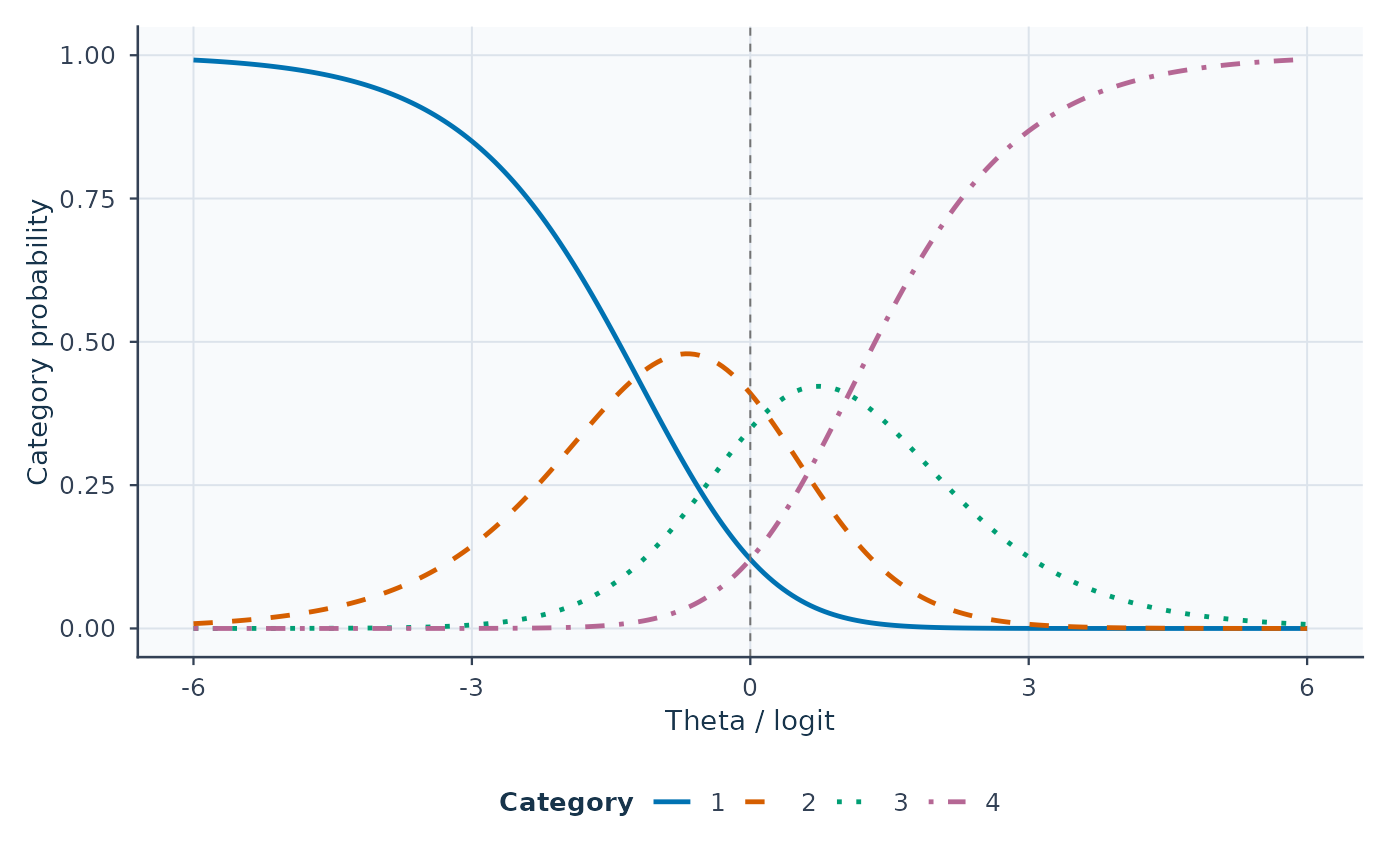The expected-score pathway draw-free data also includes pathway_long, pathway_annotations, fit_measures, fit_status, and curve_fit_status, so R users can rebuild the pathway map in ggplot2, plotly, or a report pipeline while keeping the same underfit/overfit labels used by fit_measures_table(). type = "ccc" shows category response probabilities. Multiple curve groups are faceted rather than overplotted by the native renderer, and category-specific legends use the same colours across panels. Multiple groups or more than five categories use one legend beside the plotting area; colour presets use distinct default colours beyond eight categories. For GPCM, these curves retain the estimated slope. With separate owners, each step-level/slope-level pair is a labeled curve group. Such joint profiles have no single-facet Infit/Outfit flag; inspect fit_measures or type = "fit_pathway" separately. All curve families are reference-profile curves with additive facet main effects and fitted interactions fixed at zero; the native footer and ggplot subtitle disclose that conditioning. Expected-score pathways use the same reference profile and expose the same curve_basis table. These curves do not average over the observed rater assignments or show a particular fitted interaction cell. The draw-free curve_basis, CurveBasis, and PredictorOffset fields make that conditioning explicit. type = "ccc_surface" or type = "category_surface" returns 3D-ready category-probability surface data for external rendering; it deliberately does not add a plotly/rgl dependency or replace the 2D CCC/pathway reporting figures. The returned object includes category_support, interpretation_guide, and reporting_policy tables so retained zero-frequency categories and manuscript-use boundaries remain visible to beginners. The remaining types ("facet", "person", "step", "shrinkage") provide compact location-specific displays.

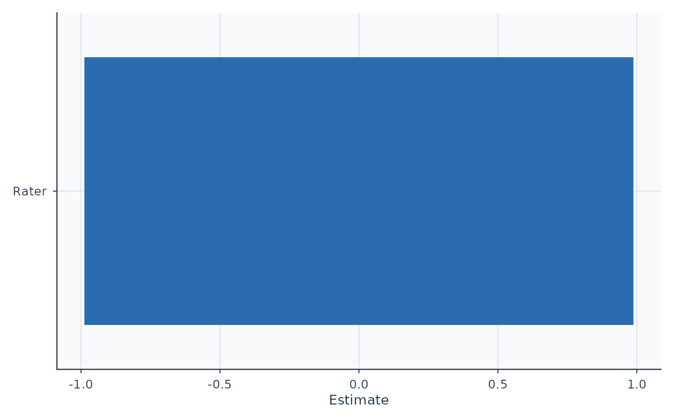
plot(fit, type = "rater_severity", facet = "Rater") orders locations and shows available normal uncertainty intervals. Pass matching diagnostics to reuse their precision metadata. The default has no magnitude bands; show_bands = TRUE explicitly adds gray guides at +/-0.5 and +/-1.0 logits. These distances from the fitted zero are not equivalence bounds, evidence of homogeneity or calibration standards. The returned data table uses numerical absolute-location ranges in Band; a common range does not imply small pairwise differences.

Use p <- plot(fit, type = "rater_severity", diagnostics = diagnostics) and plot_data() to read "data" and "notes". Intervals retain their CIUse, SE_Method and IntervalStatus; individual whisker overlap is not a contrast interval. analyze_facet_equivalence() separately examines pairwise differences with their full covariance and a prespecified practical bound in its supported MML scope. It does not use the profile's guides. The zero depends on the model constraints/anchors, so read the signed differences and their uncertainty instead of inferring quality from color. Older saved profiles retain their original colors and labels when converted with as_ggplot(); regenerate the figure from the saved fit and matching diagnostics for the new display. No refitting is needed.

Corrected JML plots

A fit with an explicit jml_correction_order uses type = "slopes" (default), "locations" or "steps". Locations show one facet, defaulting to the first declared facet. style = "points" shows estimates without intervals; "distribution" shows their empirical cumulative distribution. These displays do not classify rater quality. They support title, caption, show_title, show_notes, show_labels, sort, palette, preset, text_scale, point_size, and draw-free as_ggplot() conversion. Slopes use a reference of one; location/step displays use zero. Ordinary plot types, show_ci = TRUE, and unrelated plot controls are rejected for this estimator. The figure retains point estimates if their RootSE is unavailable; it cannot be drawn if no unambiguous point solution was obtained.

Graphics layout

Single-panel plots advance through a caller's par(mfrow = ...) or layout() arrangement and restore the style and margins they change. Native Wright maps, multi-group CCC plots, and faceted fit pathways create their own page layouts; call these outside a custom layout() arrangement. Use renderer = "facets" for a single-panel Wright map in a custom grid. A 7 by 5 inch device is a useful starting size for standalone plots; dense PCM labels benefit from a wider device. Native Wright/pathway plots warn when labels cannot be separated within the available space. Enlarge the device (for example, to 12 by 8 inches) and inspect the result; this warning concerns readability, not model fit. Abbreviated labels retain distinguishing text where possible, falling back to full names if needed. Original names remain available in the plot data. For non-Latin labels, select a graphics device and font that support the characters before plotting; the package retains the caller's font family.

Typical workflow

Fit a model with fit_mfrm().
Use plot(fit) to inspect the Wright map at a glance.
Switch to type = "pathway", "fit_pathway", "ccc", or "shrinkage" for the relevant follow-up figure, or type = "bundle" for the three-plot overview when preparing a FACETS-style summary.

Further guidance

For a plot-selection guide and extended examples, see mfrmr_visual_diagnostics and vignette("mfrmr-visual-diagnostics", package = "mfrmr").

Session plot defaults

See mfrmr_visual_diagnostics for options(mfrmr.plot_preset), argument precedence, and appearance when saving or reusing a plot.

Examples

library(mfrmr)

# Saved synthetic MML/RSM analysis of example_operational.
# For your own data, fit a model first; see ?fit_mfrm.
example_fit <- readRDS(system.file("examples", "operational-mml.rds", package = "mfrmr"))
fit <- example_fit$fit

# Run each plot command separately to inspect its figure
plot(fit) # Wright map: persons, facets, and category thresholds


# Rater severity estimates (higher means more severe in this example)
plot(fit, type = "facet", facet = "Rater")


# Probability of each score category across the ability scale
plot(fit, type = "ccc")


# Optional: get plot without printing and inspect underlying tables
wright <- plot(fit, draw = FALSE)
head(plot_data(wright, "locations"))
#> # A tibble: 6 × 39
#>   Group Label PlotType    Estimate    SE Fixed CI_Level SE_Method  PrecisionTier
#>   <fct> <chr> <chr>          <dbl> <dbl> <lgl>    <dbl> <chr>      <chr>        
#> 1 Rater R01   Facet level   -0.606 0.181 FALSE     0.95 Observati… exploratory  
#> 2 Rater R02   Facet level   -0.382 0.166 FALSE     0.95 Observati… exploratory  
#> 3 Rater R04   Facet level    0.180 0.185 FALSE     0.95 Observati… exploratory  
#> 4 Rater R05   Facet level    0.184 0.199 FALSE     0.95 Observati… exploratory  
#> 5 Rater R03   Facet level    0.212 0.179 FALSE     0.95 Observati… exploratory  
#> 6 Rater R06   Facet level    0.412 0.219 FALSE     0.95 Observati… exploratory  
#> # ℹ 30 more variables: SupportsFormalInference <lgl>, SEUse <chr>,
#> #   CIBasis <chr>, CIUse <chr>, CIEligible <lgl>, CILabel <chr>,
#> #   Measure_Source <chr>, CI_Lower <dbl>, CI_Upper <dbl>, Step <chr>,
#> #   StepIndex <int>, BoundarySeparated <lgl>, Highlighted <lgl>, XBase <dbl>,
#> #   X <dbl>, OriginalEstimate <dbl>, BelowRange <lgl>, AboveRange <lgl>,
#> #   DisplayEstimate <dbl>, DisplayLabel <chr>, OriginalCI_Lower <dbl>,
#> #   OriginalCI_Upper <dbl>, DisplayCI_Lower <dbl>, DisplayCI_Upper <dbl>, …
# Find a named judge without refitting or dropping the surrounding scale
judge <- subset(plot_data(wright, "locations"), Group == "Rater")$Label[1]
focused <- plot(fit, highlight = list(Rater = judge), draw = FALSE)
subset(plot_data(focused, "locations"), Highlighted)
#> # A tibble: 1 × 39
#>   Group Label PlotType    Estimate    SE Fixed CI_Level SE_Method  PrecisionTier
#>   <fct> <chr> <chr>          <dbl> <dbl> <lgl>    <dbl> <chr>      <chr>        
#> 1 Rater R01   Facet level   -0.606 0.181 FALSE     0.95 Observati… exploratory  
#> # ℹ 30 more variables: SupportsFormalInference <lgl>, SEUse <chr>,
#> #   CIBasis <chr>, CIUse <chr>, CIEligible <lgl>, CILabel <chr>,
#> #   Measure_Source <chr>, CI_Lower <dbl>, CI_Upper <dbl>, Step <chr>,
#> #   StepIndex <int>, BoundarySeparated <lgl>, Highlighted <lgl>, XBase <dbl>,
#> #   X <dbl>, OriginalEstimate <dbl>, BelowRange <lgl>, AboveRange <lgl>,
#> #   DisplayEstimate <dbl>, DisplayLabel <chr>, OriginalCI_Lower <dbl>,
#> #   OriginalCI_Upper <dbl>, DisplayCI_Lower <dbl>, DisplayCI_Upper <dbl>, …