
mfrmr provides estimation, diagnostics, and reporting utilities for
many-facet ordered-response measurement models: the Rasch-family RSM /
PCM route and a GPCM extension in which one selected facet supplies
level-specific discriminations. MML permits a different facet to supply
category steps; JML requires the same facet for both roles. confint.mfrm_fit()
with parm = "slopes"
supplies approximate relative-slope intervals for eligible MML fits; model
ranking and matched PCM/GPCM tests use separate checks in compare_mfrm().
mfrmr_output_guide("gpcm_capabilities") (see mfrmr_gpcm_scope) explains the supported uses.
An experimental two-family GPCM route also provides estimation and
conditional scoring, with explicit uncertainty limitations.
Native RSM/PCM conditional maximum likelihood (CML) conditions on Person
totals without assuming an ability distribution. Its separate result class
supplies structural contrast intervals through mfrm_facet_intervals(),
without Person abilities, a population SD or ordinary fit diagnostics.
See fit_mfrm() for the supported conditional estimation scope.
For assessment planning from observed scores, mfrm_g_study()
and mfrm_d_study() separate sources of variation and project
dependability for specified future rating plans. For rater feedback and
assessment decisions, mfrm_report(), interrater_agreement_table() and
classification_table() provide their respective reports, agreement
measures and fixed-plan classification summaries. These analyses have
different assumptions and uncertainty targets; follow the linked help for
the question you want to answer.
Details
Start with the complete script in the Examples section:
Load the package and example ratings with
load_mfrmr_data().Fit a model with
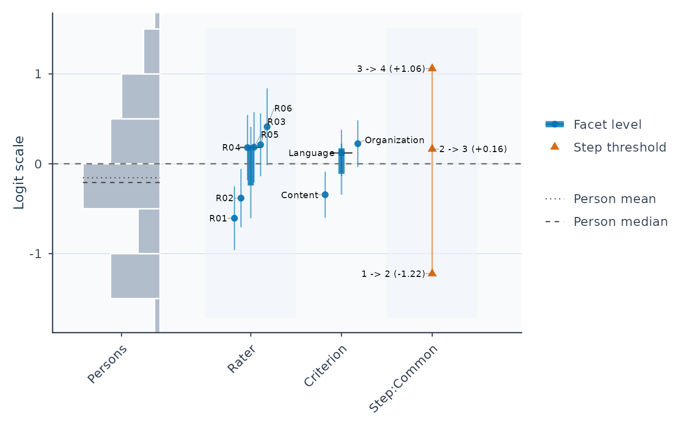
fit_mfrm().Draw the Wright map with
plot(fit).Save
results <- summary(fit)and inspectresults$person_overviewandresults$facet_overview.
Each data row is one rating event. The person, facets, and score
arguments name columns. The example uses marginal maximum likelihood
(MML) and a rating-scale model (RSM) with shared category thresholds.
head(ratings) displays the first six rows. Only Person, Rater, Criterion,
and Score are used by this model; the example's Study and Group columns
are additional labels. <- saves an object, and $ selects a named part:
results$person_overview displays one table from the saved summary.
The overview tables summarize distributions; as.data.frame(fit) returns
individual person, rater, and criterion estimates.
The assignment ratings <- load_mfrmr_data("example_operational") reads
an existing synthetic dataset supplied with mfrmr. You do not need to create
ratings first; the name on the left stores what the function returns.
Before interpreting or reporting estimates, read results$decision and
follow its NextAction. The default summary does not compute diagnostics.
For your own data, first inspect the design and score categories with
describe_mfrm_data().
Core five-step workflow
Across the package's three pillars (measurement models, G-theory assessment
planning, and rater feedback / decisions), most analyses follow five entry
points (mfrmr_output_guide("core_workflow")):
Inspect data and anchors:
describe_mfrm_data()(andreview_mfrm_anchors()when linking across waves or subsets).Fit the measurement model:
fit_mfrm(), passing either the 16 core arguments directly or a reusablespec = list(...)plus optional numericalcontrol = list(...)(see fit_mfrm_technical_details for all 33specand 21controlkeys). The samespeclist can be shared unchanged acrossdescribe_mfrm_data(),review_mfrm_anchors(),fit_mfrm(), andexport_mfrm_model().Diagnose model fit and rater effects:
diagnose_mfrm()(usediagnostic_mode = "both"for final RSM/PCM MML runs).Plan future designs under G-theory:
mfrm_g_study()andmfrm_d_study()on observed ratings (separate from latent-logit MFRM separation).Report and visualize:
mfrm_results(),mfrm_report(), andplot()(all 62plot()methods render and returnggplot2objects directly; extract underlying tables and cautions viaplot_data()).
Optional packages
The basic example below uses packages installed with mfrmr, including
ggplot2 for all plot() methods and as_ggplot(). Additional suggested
packages support particular specialist features; you do not need to install
all suggested packages to get started.
as_kable()needs knitr andas_flextable()needs flextable for their respective table formats.fit_mfrm_random_rater()needs RTMB version 2.0 or later for shared random-rater estimation.Corrected JML in
fit_mfrm(), requested withjml_correction_order, needs nleqslv to solve the adjusted equations.ordinal_logistic_table()needs ordinal for ordinal-logistic DIF.export_mfrm_model(..., format = "stan", run_cmdstan = TRUE)needs cmdstanr and a configured CmdStan installation for live MCMC sampling.
These are common examples; other optional analyses name their dependencies
in their own help. A missing-package message identifies what to install.
For example, use install.packages("flextable") if you want as_flextable().
A saved mfrm_results() bundle can be reopened with base::readRDS() and
passed to mfrm_report() without refitting or installing optional estimation
packages. Reporting reuses stored results and retains unavailable diagnostics
as unavailable. Updating an analysis or computing new diagnostics is a
separate operation and may need the original dependencies. Save the complete
bundle with base::saveRDS() and retain its matching package version/source;
see "Updating saved analyses for 0.2.4" in mfrmr_workflow_methods before
reusing older saved analyses.
Measurement scale
Native response models use the logistic metric (L-metric), with scaling
constant \(D = 1\); no extra 1.7 normal-ogive approximation factor is used.
This is distinct from choosing a normal ability distribution. See the
"Logistic metric (D = 1)" section of fit_mfrm_technical_details (linked
from fit_mfrm()) for logit interpretation with fixed or varying slopes and
comparison with other software.
Where to go next
fit_mfrm_technical_details for full equations, identification rules, numerical controls, and return-object provenance of
fit_mfrm().mfrmr_methods_reference for the question-to-calculation map, plain-language explanations and links to the methodological literature.
mfrmr_workflow_methods and
vignette("mfrmr-workflow", package = "mfrmr")for your own CSV, column mapping, input troubleshooting, and the full analysis workflow. If vignettes are not installed, start withdescribe_mfrm_data()andrecode_missing_codes().mfrmr_visual_diagnostics for choosing follow-up figures.
mfrmr_reporting_and_apa and mfrmr_reports_and_tables for reporting.
mfrmr_linking_and_dff for linking and differential facet functioning.
classification_table()for fixed-plan future classification accuracy, consistency and conditional precision under ordinary RSM/PCM calibration.mfrmr_gpcm_scope for the
GPCMextension.mfrmr_output_guide()for the broader purpose-to-function map.
A printable reference card is available at
system.file("cheatsheet", "mfrmr-cheatsheet.pdf", package = "mfrmr").
Portable fixed calibration
A saved, versioned calibration artifact can be created from an eligible
one-scale RSM or PCM MML fit under the fixed standard-normal scoring
basis. Use mfrmr_output_guide("calibration_capabilities") before extraction, then follow
mfrm_calibration_workflow to review, validate, freeze, save, load, and
score the artifact. Review the returned batch with
mfrm_calibration_score_methods before using its estimates. One-family GPCM
MML also supports an estimated intercept-only normal population, shared or
separate slope/step owners, unit weights and no anchors/interactions, subject
to conditional source and per-batch numerical scoring checks. Estimated-
population RSM/PCM and latent-regression MML remain fitted-object-only.
RSM/PCM JML supports portable post-hoc EAP with a standard-normal reference
prior, unit weights, no anchors/interactions and passing finite identified
source checks. Shared-owner GPCM JML also supports conditional portable
EAP after its joint-likelihood/curvature checks, preserving incomplete global
audits. Explicit corrected GPCM JML instead uses adjusted-equation checks
and preserves the correction order in format 5; residual calibration bias
may remain. That reference prior is not estimated by JML. Experimental
two-family GPCM MML uses format 6 with both ordered slope owners and a fixed
N(0,1) prior, separate source/batch checks and no prior overrides.
Artifact
score uncertainty is conditional on the frozen point calibration and its
recorded prior; loading validates consistency but does not authenticate an
untrusted file.
Advanced scope
After the basic route above:
the package supports latent-regression
MMLfor ordered-responseRSM/PCMmodels with a one-dimensional conditional-normal population model and explicit one-row-per-person covariates expanded throughstats::model.matrix()GPCMsupport is summarized bymfrmr_output_guide("gpcm_capabilities")(mfrmr_gpcm_scope)GPCMsupports the core fit/summary/scoring/information path, direct Wright/pathway/CCC plots, residual-PCA follow-up, and the residual-based diagnostics tables/plots as exploratory toolsposterior-predictive checks and
MCMCestimation are not available forGPCM; use external Bayesian software when they are requireddirect
GPCMdata generation throughbuild_mfrm_sim_spec(),extract_mfrm_sim_spec(), andsimulate_mfrm_data()is available when the specification carries both thresholds and slopes with the same owner; general simulation/design workflows do not support separate ownersslope-aware
fair_average_table()andestimate_bias()are available forGPCMwith explicit caveats;build_apa_outputs(),build_visual_summaries(),run_qc_pipeline(),build_mfrm_manifest(),build_mfrm_replay_script(), andexport_mfrm_bundle()are available as caveated partial reporting/export surfaces; score-side FACETS compatibility remains limited, and fully arbitrary-facet planning is outside the documented planning scopepredict_mfrm_population()remains a scenario-level forecast helper and should not be described as the latent-regression estimator itselfthe current simulation/planning layer remains role-based for two non-person facets rather than fully arbitrary-facet planning, with boundaries exposed through planner metadata such as
planning_scope,planning_constraints, andplanning_schemalatent-class mixture models and response-time / careless-rating adjustment are not estimated by mfrmr; use residual, person-fit, local-dependence, and rater-drift diagnostics as screening layers rather than as mixture-model substitutes
Equal weighting versus GPCM
The package's operational reference route is the Rasch-family
RSM / PCM branch. That route enforces fixed discrimination and therefore
preserves an equal-weighting scoring interpretation across observed ratings.
GPCM is supported because some users want a slope-aware model-
comparison or sensitivity layer inside the same many-facet workflow. However,
the package does not treat GPCM as a universal replacement for the
Rasch-family route. A better fit under GPCM should be read as evidence
about discrimination-based reweighting, not as an automatic reason to
discard the equal-weighting model.
Observation weights are a different concept again. Optional Weight
columns change how observed rating events enter estimation and summaries, but
they do not create a free-form facet-weighting scheme and do not alter the
fixed-discrimination meaning of RSM / PCM.
Public entry map:
First-screen results:
mfrm_results(),summary(res)$next_actions, andmfrmr_output_guide("entry")Interactive exploration:
mfrm_results_interactive()only when prompts are explicitly wanted at the console
Function families:
Model fitting:
fit_mfrm(),summary.mfrm_fit(),plot.mfrm_fit()Legacy-compatible workflow wrapper:
run_mfrm_facets(),run_mfrm_facets()Diagnostics:
diagnose_mfrm(),summary(diag),analyze_residual_pca(), plot(x, type = "residual_pca")Bias and interaction:
estimate_bias(),estimate_all_bias(),summary(bias),bias_interaction_report(), plot(x, type = "bias")Differential functioning:
analyze_dff(),mantel_haenszel_table()for separately matched binary responses,ordinal_logistic_table()for matched cumulative-logit comparisons,dif_interaction_table(), plot(x, type = "heatmap"),dif_report()Design simulation:
build_mfrm_sim_spec(),extract_mfrm_sim_spec(),simulate_mfrm_data(),simulate_mfrm_recovery(),assess_mfrm_recovery(),evaluate_mfrm_design(),evaluate_mfrm_signal_detection(),predict_mfrm_population(),predict_mfrm_units(),sample_mfrm_plausible_values()(including fit-derived empirical / resampled / skeleton-based simulation specifications; fitted-object posterior scoring supportsMMLfits directly, latent-regressionMMLfits through the fitted population model when scored units also provide one-row-per-person background data, andJMLfits through a post hoc reference-prior EAP layer; fit-derived simulation specifications also support directGPCMdata generation, recovery checks, role-based design evaluation, population forecasting, diagnostic-screening, and signal-detection helpers with documented caveats; curve reports, graph-only exports, fair-average tables, and bias screening are also available forGPCMwith documented caveats)Reporting:
build_apa_outputs(),build_visual_summaries(),reporting_checklist(),apa_table()for the fullRSM/PCMroute;GPCMuses these as caveated partial surfaces and retains direct table, plot, checklist, and summary-appendix routesWeighting review:
compare_mfrm(),build_weighting_review(),build_model_choice_review(),compute_information(), plot(x)Case review:
build_misfit_casebook(), plot(x, type = "unexpected"), plot(x, type = "displacement"), plot(x, type = "marginal_fit"), plot(x, type = "marginal_pairwise")Linking and scale maintenance:
review_mfrm_anchors(),detect_anchor_drift(),build_equating_chain(),build_linking_review(), plot(x)Dashboards:
facet_quality_dashboard(), plot(x, type = "facet_dashboard")Export / reproducibility:
build_mfrm_manifest(),build_mfrm_replay_script(),build_conquest_overlap_bundle(),normalize_conquest_overlap_exports(), file input throughnormalize_conquest_overlap_tables(input = "files"),normalize_conquest_overlap_tables(),review_conquest_overlap(),export_mfrm_bundle()for the diagnostics-compatible Rasch-family route;GPCMsupports caveated partial manifest, replay, and bundle output as well asexport_summary_appendix()Equivalence:
analyze_facet_equivalence(), plot(x, type = "facet_equivalence")Data and anchors:
describe_mfrm_data(),review_mfrm_anchors(),make_anchor_table(),load_mfrmr_data()
Data interface:
Input analysis data is long format (one row per observed rating).
Required columns are one person column, one ordered score column, and one or more non-person facet columns named in
facets = c(...).Score values should be ordered integer categories. Binary
0/1or1/2input is supported as the two-category Rasch-family special case; by contrast, fractional score values should be recoded before fitting rather than relying on automatic coercion.If
keep_original = FALSE, unused intermediate categories are collapsed to a contiguous internal scale and the mapping is stored infit$prep$score_map.If the intended scale has unused boundary categories, such as a 1-5 scale with only 2-5 observed, set
rating_min = 1, rating_max = 5so the zero-count boundary category remains explicit in the data-support review. A missing boundary remains review evidence for the separate element- boundary contract. If unused intermediate categories should remain in the original scale, setkeep_original = TRUE; a retained zero-count internal category in a polytomous fitted ladder creates an unsupported adjacent- step contrast, andfit_mfrm()returns a structured pre-optimization error.summary(describe_mfrm_data(...))reports retained zero-count categories inNotes, printedCaveats, and$caveats;summary(fit)carries full structured rows into printedCaveatsand$caveats, withKey warningsas a short triage subset. Summary-table exports route those rows throughscore_category_caveatsoranalysis_caveats.A category can be observed globally but unused by one rater or other facet level. Review that local pattern with
data_quality_report()rather than treating it as a globally missing step or an automatic reason to selectGPCM.Optional columns such as
Subset,Weight, andGroupsupport linking, weighted analysis, and fairness-focused follow-up workflows.Packaged synthetic data is available via
load_mfrmr_data()ordata(). Uselist_mfrmr_data(details = TRUE)to distinguish the applied teaching, idealized, planted-effect, and larger sparse-design datasets.
Interpreting output
Core object classes are:
mfrm_fit: fitted model parameters and metadata.mfrm_diagnostics: fit, facet-level reliability, and flag diagnostics, plus inter-rater agreement when one facet is treated as a rater facet.mfrm_bias: interaction bias estimates.mfrm_dff/mfrm_dif: differential-functioning contrasts and screening summaries.mfrm_population_prediction: scenario-level forecast summaries for one future design.mfrm_unit_prediction: posterior summaries for future or partially observed persons under the fitted scoring basis.mfrm_plausible_values: posterior draws for future or partially observed persons under the fitted scoring basis.mfrm_bundlefamilies: summary/report bundles and draw-free plot data.
Typical workflow
Prepare long-format data.
Fit with
fit_mfrm().For
RSM/PCM, diagnose withdiagnose_mfrm()and preferdiagnostic_mode = "both"for finalMMLruns.For
RSM/PCM, runanalyze_dff()orestimate_bias()when fairness or interaction questions matter;GPCMalso supportsestimate_bias()as a conditional screening review.For
RSM/PCM, report withbuild_apa_outputs()andbuild_visual_summaries().For design planning, move to
build_mfrm_sim_spec(),evaluate_mfrm_design(),mfrm_generalizability(),mfrm_d_study(), andpredict_mfrm_population().GPCMalso supports direct simulation viaextract_mfrm_sim_spec()/simulate_mfrm_data()and caveated role-basedevaluate_mfrm_design()/predict_mfrm_population()routes. Those helpers assume two non-person facet roles even though the estimation core supports arbitrary facet counts. Treatevaluate_mfrm_design()as Monte Carlo design evaluation, and usemfrm_d_study()for analytic G/Phi design projections. Always read theIdentificationStatus,GStatus, andPhiStatuscolumns before reporting those projections; boundary or singular mixed-model fits are design-identification warnings, not high-stakes-ready reliability evidence.predict_mfrm_population()remains the scenario-level forecast helper, not the latent-regression estimator.For future-unit scoring, retain an
MMLcalibration when you want the fitted marginal model directly, use an active latent-regressionMMLfit when scored units also provide one-row-per-person background data, or use aJMLcalibration when a post hoc fitted-object EAP layer is acceptable; then score withpredict_mfrm_units()orsample_mfrm_plausible_values().For
GPCM, usesummary.mfrm_fit(),diagnose_mfrm(),analyze_residual_pca(),predict_mfrm_units(),sample_mfrm_plausible_values(),compute_information(), plot(x, type = "qc"),plot.mfrm_fit(),category_structure_report(),category_curves_report(), graph-onlyfacets_output_file_bundle(), direct simulation-spec generation/data generation, recovery checks,fair_average_table(),estimate_bias(), and the residual-based table helpers with their documented caveats. Caveated APA/QC/export bundles and exploratory linking review plus role-based design evaluation, population forecasting, diagnostic-screening, and signal-detection helpers are available, while full score-side FACETS review, posterior-predictive checks, andMCMCestimation are not available forGPCM. Usemfrmr_output_guide("gpcm_capabilities")(mfrmr_gpcm_scope) as the formal boundary statement.
Model formulation
The Rasch-family branch used by RSM and PCM extends the basic Rasch
model by incorporating multiple measurement facets into a single additive
linear predictor on the log-odds scale.
RSM/PCM adjacent-category equation
For an observation where person \(n\) with ability \(\theta_n\) is rated by rater \(j\) with severity \(\delta_j\) on criterion \(i\) with difficulty \(\beta_i\), the probability of observing category \(k\) (out of \(K\) ordered categories) is:
$$P(X_{nij} = k \mid \theta_n, \delta_j, \beta_i, \tau) = \frac{\exp\bigl[\sum_{s=1}^{k}(\theta_n - \delta_j - \beta_i - \tau_s)\bigr]} {\sum_{c=0}^{K}\exp\bigl[\sum_{s=1}^{c}(\theta_n - \delta_j - \beta_i - \tau_s)\bigr]}$$
where \(\tau_s\) are the Rasch-Andrich threshold (step) parameters in the
RSM reference case and
\(\sum_{s=1}^{0}(\cdot) \equiv 0\) by convention. Additional facets
enter as additive terms in the linear predictor
\(\eta = \theta_n - \delta_j - \beta_i - \ldots\).
This additive predictor generalises to any number of facets; the
facets argument to fit_mfrm() accepts an arbitrary-length
character vector.
Rating Scale Model (RSM)
Under the RSM (Andrich, 1978), all levels of the step facet share a single set of threshold parameters \(\tau_1, \ldots, \tau_K\).
Partial Credit Model (PCM)
Under the PCM (Masters, 1982), each level of the designated step_facet
has its own threshold vector on the package's common observed score scale.
In the current implementation, threshold locations may vary by step-facet
level, but the fitted score range is defined by one global category
set taken from the observed data.
Generalized Partial Credit Model (GPCM)
With one slope family under GPCM (Muraki, 1992), the adjacent-category partial-credit
kernel is multiplied by a positive slope \(\alpha_g\) for the designated
slope-facet level \(g\):
$$\ln\frac{P(X_{nij} = k)}{P(X_{nij} = k-1)} = \alpha_g(\theta_n - \delta_j - \beta_i - \tau_{hk}).$$
MML allows a slope owner \(g\) distinct from the step owner \(h\);
JML requires slope_facet == step_facet. Slopes are identified on the log
scale with geometric mean 1. This makes
GPCM a slope-aware sensitivity/extension route, not a replacement for the
equal-weighting RSM/PCM interpretation.
A separate provisional two-family MML route fits the multiplicative
Uto–Ueno equation with explicit fixed-N(0,1) identification and allows
additional fixed additive facets. Step ownership and the noncentered
location facet are explicit. The named reference family's slopes have
geometric mean one and the other family's slopes are free. Fixed-grid EM and adaptive
direct MML supply summaries and conditional fitted curves without intervals.
Both support separately checked experimental component log-Wald and
location/contrast intervals and descriptive posterior residuals; component
profiles preserve the fitted fixed-grid or adaptive integration and require
separate numerical checks. predict_mfrm_units() and the portable
calibration workflow supply experimental conditional new-Person EAP and
posterior intervals, excluding calibration uncertainty. Coverage and
population transport remain unqualified. The one-family diagnostic and
inference routes below do not apply to it. See the
"Two slope families" section of fit_mfrm_technical_details (linked from
fit_mfrm()). Unit slopes reduce to the
equal-discrimination PCM kernel.
Under default one-family MML, an intercept-only person distribution
\(N(\beta_0,\sigma^2)\) is estimated. The geometric-mean-one slopes are
relative discriminations and \(\sigma\alpha_g\) are their equivalent
fixed-latent-standard-deviation values, so the conventional common
discrimination degree of freedom is retained. The legacy
gpcm_mml_identification = "fixed_standard_normal" mode fixes both
\(\sigma=1\) and the slope geometric mean to one and is therefore a
narrower relative-discrimination model. Under JML, geometric-mean-one is
required to resolve the scale of jointly estimated person coordinates.
The former "bounded" label described limited model/workflow scope, not
finite optimizer box constraints. Use GPCM with explicit scope restrictions.
The GPCM JML objective is unpenalized.
Certified extreme-person or facet recession is reported through typed
primary boundary results; a finite optimizer iterate is retained only as a
numerical trace and is not a finite JML maximum.
Ordered-response scope
The implemented response-model scope is ordered categorical only.
Binary responses are the \(K = 1\) special case of the same formulation,
so they are handled through the ordinary ordered-score interface. This means
mfrmr supports ordered binary and ordered polytomous data under RSM and
PCM, plus GPCM with one designated slope_facet and, under MML,
a possibly different step_facet. Unordered
nominal/multinomial response models are outside the documented model scope,
as are Poisson, negative-binomial, and grouped binomial-trial count-response
families. A positive observation weight weights the conditional
ordered-rating contribution; it is not a general collapsed-person frequency
table and does not change the response family or model dependence among
replicated ratings. Under MML, powering conditional responses within one
Person is not the same as replicating a complete Person pattern after
marginalization. Consequently, integer count values supplied as scores are
modeled as ordered category codes, not as counts from a Poisson or related
distribution.
Estimation methods
Marginal Maximum Likelihood (MML)
MML integrates over the person ability distribution using Gauss-Hermite quadrature, in the broader marginal-likelihood framework introduced by Bock & Aitkin (1981) for IRT:
$$L = \prod_{n} \int P(\mathbf{X}_n \mid \theta, \boldsymbol{\delta}) \, \phi(\theta) \, d\theta \approx \prod_{n} \sum_{q=1}^{Q} w_q \, P(\mathbf{X}_n \mid \theta_q, \boldsymbol{\delta})$$
where \(\phi(\theta)\) is the assumed normal prior and \((\theta_q, w_q)\) are quadrature nodes and weights. Person estimates are obtained post-hoc via Expected A Posteriori (EAP):
$$\hat{\theta}_n^{\mathrm{EAP}} = \frac{\sum_q \theta_q \, w_q \, L(\mathbf{X}_n \mid \theta_q)} {\sum_q w_q \, L(\mathbf{X}_n \mid \theta_q)}$$
MML does not estimate one fixed person parameter per respondent and therefore avoids that JML incidental-parameter mechanism. Its structural inference is nevertheless conditional on the specified population distribution, response model, quadrature approximation, and regularity conditions; it is not an automatic small-sample guarantee.
Note: Bock & Aitkin (1981) is the canonical citation for the
Gauss-Hermite-quadrature MML framework. The default mfrmr engine
(mml_engine = "direct") optimises this marginal log-likelihood by
direct gradient methods (BFGS / L-BFGS-B), not by Bock & Aitkin's
signature EM algorithm. The "em" and "hybrid" engines do follow
the EM template but use the selected gradient-based M-step rather than
B&A's probit IRLS,
because the target is the polytomous Rasch family rather than B&A's
2PL probit model.
Conditional Maximum Likelihood (CML)
For supported RSM/PCM models, CML conditions on each Person's total and
observed assignments, removing ability parameters without specifying their
population distribution. A generalized elementary-symmetric-function
recursion evaluates the conditional likelihood and information. Identification
and finite-MLE checks precede structural contrast intervals; their Wald
interpretation is asymptotic, not a general finite-sample coverage guarantee.
The separate mfrm_cml_fit and comparison-only results supply no Person
abilities or population SD. Use mfrm_facet_intervals() for their
native-scale intervals. CML does not support GPCM or ordinary diagnostics.
Joint Maximum Likelihood (JML)
JML estimates all person and facet parameters simultaneously as fixed
effects by maximising the joint log-likelihood
\(\ell(\boldsymbol{\theta}, \boldsymbol{\delta} \mid \mathbf{X})\)
directly. It does not assume a parametric person distribution, which
can be advantageous when the population shape is strongly non-normal.
Its incidental-parameter concern is not simply a small-person-sample issue:
structural-parameter bias can persist as the number of persons increases
when the number of ratings or items per person remains fixed (Neyman &
Scott, 1948).
The package still accepts "JMLE" as a backward-compatible alias, but
user-facing summaries and documentation use "JML" as the public label.
See fit_mfrm() for practical guidance on choosing an estimator. General
GPCM inference uses MML; JML remains useful for descriptive point estimates
and FACETS comparisons.
Strict marginal diagnostics
For RSM / PCM, diagnose_mfrm(..., diagnostic_mode = "both")
returns two complementary targets: the legacy residual / EAP
diagnostics and a marginal_fit layer whose expected counts and
pairwise summaries are integrated over the posterior quadrature
bundle rather than plugged in at the EAP point. The screen is
structured as limited-information evidence (Orlando & Thissen,
2000; Haberman & Sinharay, 2013; Sinharay & Monroe, 2025), not as
an omnibus accept / reject test, and it complements rather than
replaces separation / reliability and inter-rater agreement
summaries. The full derivation, with notation and pairwise
local-dependence events, lives in
online MML and marginal-fit guide.
Statistical background
Key statistics reported throughout the package:
Infit (Information-Weighted Mean Square)
Weighted average of squared standardized residuals, where weights are the model-based variance of each observation:
$$\mathrm{Infit}_j = \frac{\sum_i Z_{ij}^2 \, \mathrm{Var}_i \, w_i} {\sum_i \mathrm{Var}_i \, w_i}$$
Expected value is 1.0 under model fit. Values below 0.5 suggest overfit (Mead-style responses); values above 1.5 suggest underfit (noise or misfit). Infit is most sensitive to unexpected patterns among on-target observations (Wright & Masters, 1982).
Note: The 0.5–1.5 range is the general "productive for measurement" band given by Linacre (2002, RMT 16(2), 878). Context-specific bands come from Wright & Linacre (1994, RMT 8(3), 370): 0.8–1.2 for high-stakes MCQ, 0.7–1.3 for run-of-the-mill MCQ, 0.6–1.4 for rating-scale surveys, 0.5–1.7 for clinical observation, and 0.4–1.2 for judged performance. See also Bond & Fox (2015) for textbook summaries of these conventions.
Outfit (Unweighted Mean Square)
Simple average of squared standardized residuals:
$$\mathrm{Outfit}_j = \frac{\sum_i Z_{ij}^2 \, w_i}{\sum_i w_i}$$
Same expected value and flagging thresholds as Infit, but more sensitive to extreme off-target outliers (e.g., a high-ability person scoring the lowest category).
ZSTD (Standardized Fit Statistic)
Wilson-Hilferty (1931) cube-root transformation that converts the mean-square chi-square ratio to an approximate standard normal deviate:
$$\mathrm{ZSTD} = \frac{\mathrm{MnSq}^{1/3} - (1 - 2/(9\,\mathit{df}))} {\sqrt{2/(9\,\mathit{df})}}$$
Values near 0 indicate expected fit. The conventional
\(|\mathrm{ZSTD}| \ge 2\) and \(|\mathrm{ZSTD}| \ge 3\) cutoffs are heuristic
two- and three-standard-deviation reference bands (Wright & Linacre, 1994;
see also Wilson & Hilferty, 1931), not calibrated 5\
tests. Parameter estimation, sparse cells, the selected df convention, and
repeated screening across elements all affect that interpretation.
Diagnostics default to FACETS fourth-moment df, admitting df > 0 and
capping ZSTD at +/-9. The explicit engine convention withholds df < 1.
whexact = FALSE uses the expression above (FACETS YES); TRUE removes
its additive q/3 term (FACETS NO). Both use a cube root. The former linear
TRUE transformation is available only as whexact = "legacy_linear".
Residual basis under MML vs JMLE engines
For method = "MML" fits, the standardized residuals behind Infit,
Outfit, and ZSTD are evaluated at EAP person measures, which are
shrunken toward the population mean. JMLE engines such as FACETS
evaluate the same formulas at unshrunken JMLE estimates, so MnSq and
ZSTD values are not numerically interchangeable across the two residual
bases, most visibly for extreme-scoring persons. Use method = "JML"
when an external FACETS fit comparison requires a JMLE-style residual
basis, and see facets_guide() for the separate
standardization-side df/ZSTD conventions.
PTMEA (Point-Measure Correlation)
Pearson correlation between observed scores and estimated person measures within each facet level. A positive value is directionally consistent with the fitted orientation, but it is not a confirmatory test of alignment. A negative value prompts review of orientation, response patterns, and model specification; it does not by itself establish a scoring error.
Separation
Package-reported separation is the ratio of adjusted true standard deviation to root-mean-square measurement error:
$$G = \frac{\mathrm{SD}_{\mathrm{adj}}}{\mathrm{RMSE}}$$
where \(\mathrm{SD}_{\mathrm{adj}} =
\sqrt{\mathrm{ObservedVariance} - \mathrm{ErrorVariance}}\). Higher values
indicate the facet discriminates more statistically distinct levels along the
measured variable. In mfrmr, Separation is the model-based value and
RealSeparation provides a more conservative companion based on RealSE.
Reliability
$$R = \frac{G^2}{1 + G^2}$$
Analogous to Cronbach's alpha or KR-20 for the reproducibility of element
ordering. In mfrmr, Reliability is the model-based value and
RealReliability gives the conservative companion based on RealSE. For
MML, these are anchored to observed-information ModelSE
estimates for non-person facets; JML keeps them as exploratory summaries.
The facet's role determines the interpretation. High Person separation reliability indicates distinguishable abilities. High rater separation reliability indicates distinguishable severities, not agreement between raters. When raters are intended to be interchangeable, reliable severity differences merit review rather than a high-reliability quality label. Low rater separation reliability can also result from imprecise estimates; it does not establish agreement or equivalence. The index neither tests every rater pair nor quantifies the practical size of severity differences. Its Person interpretation is analogous to test reliability, but it is not numerically identical to Cronbach's alpha.
For the person facet under MML, the same \(G\) and \(R\) formulas
are applied to EAP person measures with posterior SDs in the error slot.
EAP measures are shrunken, so their observed variance is already deflated
(approximately the true variance times the reliability), and subtracting
the mean posterior variance deflates it again. The reported MML person
separation/reliability is therefore a conservative summary: it is
systematically lower than the IRT empirical-reliability convention
\(\mathrm{Var}(\mathrm{EAP}) / (\mathrm{Var}(\mathrm{EAP}) +
\overline{\mathrm{PSD}^2})\) and is not numerically comparable to
JMLE-based person separation reliability from FACETS. The gap is small
when measurement is precise and grows as precision drops. Person rows can
still carry the model-based precision tier because posterior SDs are
model-based quantities; that tier describes the SE source, not FACETS
comparability. Use method = "JML" when a FACETS-style person separation
table is required, and treat MML person rows as conservative summaries.
This is a Rasch/FACETS-style separation reliability on the fitted logit
scale, not an intra-class correlation. Use compute_facet_icc() only when
you want the complementary random-effects variance-share view on the
observed-score scale; for non-person facets, large ICC values indicate
systematic facet variance rather than desirable measurement reliability.
Strata
Number of statistically distinguishable groups of elements:
$$H = \frac{4G + 1}{3}$$
Three or more strata are commonly used as a practical target (Wright & Masters, 1982), but in this package the estimate inherits the same approximation limits as the separation index.
Key references
Andrich, D. (1978). A rating formulation for ordered response categories. Psychometrika, 43, 561–573.
Bond, T. G., & Fox, C. M. (2015). Applying the Rasch model (3rd ed.). Routledge.
Bock, R. D., & Aitkin, M. (1981). Marginal maximum likelihood estimation of item parameters: Application of an EM algorithm. Psychometrika, 46, 443–459.
Burnham, K. P., & Anderson, D. R. (2002). Model selection and multimodel inference: A practical information-theoretic approach (2nd ed.). Springer. (AIC / BIC weights and Delta-IC bands used by
compare_mfrm().)Drasgow, F., Levine, M. V., & Williams, E. A. (1985). Appropriateness measurement with polychotomous item response models and standardized indices. British Journal of Mathematical and Statistical Psychology, 38(1), 67–86. (Source for the
lzperson-fit statistic implemented incompute_person_fit_indices().)Haberman, S. J., & Sinharay, S. (2013). Generalized residuals for general models for contingency tables with application to item response theory. Journal of the American Statistical Association, 108, 1435–1444.
Eckes, T. (2005). Examining rater effects in TestDaF writing and speaking performance assessments: A many-facet Rasch analysis. Language Assessment Quarterly, 2, 197–221.
Muraki, E. (1992). A generalized partial credit model: Application of an EM algorithm. Applied Psychological Measurement, 16(2), 159–176. (Source for the GPCM response-probability kernel used by the package's bounded
fit_mfrm(model = "GPCM")route. The slope-awarefair_average_table()andestimate_bias()extensions are package-specific, caveated adaptations built from that kernel, not procedures proposed in Muraki 1992.)Muraki, E. (1993). Information functions of the generalized partial credit model. Applied Psychological Measurement, 17(4), 351–363. (Companion paper to Muraki 1992 that derives the GPCM item information identity \(I_j(\theta) = D^2 a_j^2 \mathrm{Var}(T \mid \theta)\) via Samejima's (1974) polytomous information formula. This is the canonical reference for
compute_information()underGPCM.)Samejima, F. (1974). Normal ogive model on the continuous response level in the multidimensional latent space. Psychometrika, 39, 111–121. (General polytomous information formula that Muraki 1993 specializes to the GPCM.)
Snijders, T. A. B. (2001). Asymptotic null distribution of person fit statistics with estimated person parameter. Psychometrika, 66(3), 331–342. (Source for the
lz_starcorrection incompute_person_fit_indices()when person estimates come from the JML/fixed-effect route. MML/EAP person scores are left uncorrected because EAP does not satisfy the Snijders estimating-equation setup.)Linacre, J. M. (1989). Many-facet Rasch measurement. MESA Press.
Linacre, J. M. (2002). What do Infit and Outfit, mean-square and standardized mean? Rasch Measurement Transactions, 16(2), 878.
Masters, G. N. (1982). A Rasch model for partial credit scoring. Psychometrika, 47, 149–174.
Orlando, M., & Thissen, D. (2000). Likelihood-based item-fit indices for dichotomous item response theory models. Applied Psychological Measurement, 24, 50–64.
Orlando, M., & Thissen, D. (2003). Further investigation of the performance of S-X2: An item fit index for use with dichotomous item response theory models. Applied Psychological Measurement, 27, 289–298.
Sinharay, S., Johnson, M. S., & Stern, H. S. (2006). Posterior predictive assessment of item response theory models. Applied Psychological Measurement, 30, 298–321.
Sinharay, S., & Monroe, S. (2025). Assessment of fit of item response theory models: A critical review of the status quo and some future directions. British Journal of Mathematical and Statistical Psychology, 78, 711–733.
Wright, B. D., & Masters, G. N. (1982). Rating scale analysis. MESA Press.
Wright, B. D., & Linacre, J. M. (1994). Reasonable mean-square fit values. Rasch Measurement Transactions, 8(3), 370.
Wilson, E. B., & Hilferty, M. M. (1931). The distribution of chi-square. Proceedings of the National Academy of Sciences of the United States of America, 17(12), 684-688.
Model selection
RSM vs PCM
The Rating Scale Model (RSM; Andrich, 1978) assumes all levels of the
step facet share identical threshold parameters. The Partial Credit
Model (PCM; Masters, 1982) allows each level of the step_facet to have
its own set of thresholds on the package's shared observed score scale.
Use RSM when the rating rubric is identical across all items/criteria;
use PCM when category boundaries are expected to vary by item or criterion.
In the current implementation, PCM assumes one common observed score
support across the fitted data, so it should not be described as a fully
mixed-category model with arbitrary item-specific category counts.
MML, CML and JML
Marginal Maximum Likelihood (MML) integrates over the person ability
distribution using Gauss-Hermite quadrature and does not directly estimate
person parameters; person estimates are computed post-hoc via Expected A
Posteriori (EAP). Joint Maximum Likelihood (JML) estimates all person
and facet parameters simultaneously as fixed effects; "JMLE" remains a
backward-compatible alias.
Estimator choice should follow the inferential target and assumptions. MML avoids estimating one fixed effect per person, but its structural inference depends on the specified population distribution and response model. JML does not assume a parametric person distribution and can be lighter computationally, but structural-parameter bias can persist as the number of persons increases when the number of ratings or items per person remains fixed. Sample size alone therefore does not determine the preferred route. For supported RSM/PCM structural contrasts, CML instead conditions out Person ability without a population model. It estimates neither abilities nor a population SD; same-fit population-SD standardization requires MML.
See fit_mfrm() for usage.
Fixed-calibration scoring after fitting
predict_mfrm_units() and sample_mfrm_plausible_values() score future or
partially observed persons on a quadrature grid under the fitted scoring
basis. For ordinary MML fits, these summaries inherit the fitted marginal
calibration directly. For latent-regression MML fits, they use the fitted
one-dimensional conditional normal population model and therefore require
one-row-per-person background data for the scored units when the fitted
population model includes covariates. Intercept-only latent-regression fits
(population_formula = ~ 1) can reconstruct that minimal person table from
the scored person IDs. For JML fits, mfrmr uses the fitted facet and
step parameters together with a standard normal reference prior introduced
only for the post hoc scoring layer. This is useful for practical
fixed-scale scoring, but it should still be described as a limited
approximation rather than as full ConQuest-style population modeling.
ConQuest overlap
The package supports a scoped latent-regression MML model, but
the overlap with ConQuest should still be described conservatively. The
documented comparison is binary RSM / PCM, one latent dimension,
exactly one item facet, complete rectangular responses, and exactly one
numeric person covariate beyond the intercept in a conditional-normal person
population model. This is a scoped file-based comparison, not a claim of
broad ConQuest numerical equivalence for polytomous, multidimensional,
incomplete, or arbitrary imported designs.
Author
Maintainer: Ryuya Komuro ryuya.komuro.c4@tohoku.ac.jp (ORCID) [copyright holder]
Authors:
Ryuya Komuro ryuya.komuro.c4@tohoku.ac.jp (ORCID) [copyright holder]
Examples
# Load the package
library(mfrmr)
# Load example ratings and look at the first six rows
ratings <- load_mfrmr_data("example_operational")
head(ratings)
#> Study Person Rater Criterion Score Group
#> 1 OperationalExample P001 R01 Language 4 A
#> 2 OperationalExample P001 R01 Organization 2 A
#> 3 OperationalExample P001 R02 Content 4 A
#> 4 OperationalExample P001 R02 Language 3 A
#> 5 OperationalExample P001 R02 Organization 2 A
#> 6 OperationalExample P002 R01 Content 3 A
# Fit the model
fit <- fit_mfrm(
data = ratings,
person = "Person",
facets = c("Rater", "Criterion"),
score = "Score",
rating_min = 1, rating_max = 4, category_policy = "preserve",
method = "MML",
model = "RSM"
)
# Plot the results (Wright map)
plot(fit)
 # Save the summary, then display its tables
results <- summary(fit)
results$person_overview # One row summarizing person ability estimates
#> # A tibble: 1 × 11
#> Persons DistributionN ReviewExcludedExtremeE…¹ EstimateUse Mean SD Median
#> <int> <int> <int> <chr> <dbl> <dbl> <dbl>
#> 1 48 48 0 source_fit… -0.155 0.824 -0.208
#> # ℹ abbreviated name: ¹ReviewExcludedExtremeEAPs
#> # ℹ 4 more variables: Min <dbl>, Max <dbl>, Span <dbl>, MeanPosteriorSD <dbl>
results$facet_overview # One row per facet: number of levels, mean, SD, range
#> # A tibble: 2 × 7
#> Facet Levels MeanEstimate SDEstimate MinEstimate MaxEstimate Span
#> <chr> <int> <dbl> <dbl> <dbl> <dbl> <dbl>
#> 1 Criterion 3 0 0.302 -0.344 0.224 0.568
#> 2 Rater 6 -4.64e-18 0.399 -0.606 0.412 1.02
# Check the interpretation status and recommended next step
results$decision
#> Interpretation
#> 1 Fit-readiness requirements satisfied; formal precision review required
#> FormalInference FitReadiness
#> 1 No ready
#> Why
#> 1 Formal precision support has not been evaluated. These checks assess numerical readiness and the requested precision method under the specified model; they do not establish model adequacy or finite-sample coverage for this design.
#> NextAction
#> 1 Run `diagnose_mfrm()` and pass its result as `diagnostics =` to evaluate formal precision support; fit readiness alone is not a formal-inference decision.