Convert draw-free mfrmr plot data to ggplot2

as_ggplot() is an optional renderer for an mfrm_plot_data object or an object whose plot() method supports draw = FALSE. Base graphics remain the default; the returned ggplot can be restyled or composed downstream.

Usage

as_ggplot(x, type = NULL, component = NULL, ...)

# Default S3 method
as_ggplot(x, type = NULL, component = NULL, ...)

# S3 method for class 'mfrm_design_evaluation'
as_ggplot(x, type = NULL, component = NULL, ...)

# S3 method for class 'mfrm_design_evaluation_plot_data'
as_ggplot(x, type = NULL, component = NULL, ...)

# S3 method for class 'mfrm_signal_detection'
as_ggplot(x, type = NULL, component = NULL, ...)

# S3 method for class 'mfrm_signal_detection_plot_data'
as_ggplot(x, type = NULL, component = NULL, ...)

# S3 method for class 'mfrm_plot_data'
as_ggplot(x, type = NULL, component = NULL, ...)

# S3 method for class 'mfrm_slope_intervals'
as_ggplot(x, type = NULL, component = NULL, ...)

# S3 method for class 'mfrm_curve_intervals'
as_ggplot(x, type = NULL, component = NULL, ...)

# S3 method for class 'mfrm_gpcm_bootstrap'
as_ggplot(x, type = NULL, component = NULL, ...)

# S3 method for class 'mfrm_results'
as_ggplot(x, type = NULL, component = NULL, ...)

Arguments

x: An mfrm_plot_data object, or an mfrmr object with a draw-free plot method. Corrected-JML slope, location and step plots retain their point or cumulative-distribution view, labels, reference and interpretation note; conversion does not add confidence intervals.
type: Optional plot type passed to plot() for a non-plot-data input. A saved plot-data input already selects a view and rejects type.
component: Optional tabular payload component to convert.
...: Arguments passed to the draw-free plot method. CCC conversion additionally accepts slope_aes, facet_by, and show_overlay. A saved mfrm_plot_data object already contains its view and display settings: it rejects extra arguments (except those three CCC controls for a complete CCC view). To change the level or source plot settings, create a new payload from the fitted model or statistical result. For appearance changes after conversion, use ggplot tools such as ggplot2::labs(title = NULL).

Value

A ggplot2 plot object, with a mfrmr_notes attribute when the source plot payload contains a notes table. Paired Wright/CCC payloads from plot_compare_mfrm() retain their selected comparison or difference view, group selection and monochrome panel policy.

Details

Bubble conversion uses the saved radii, facet colours, facet order and reference lines. It preserves relative circle radii, rather than replacing them with equal-sized points. Base circles use plot units; ggplot point sizes use physical units, so absolute sizes need not match across devices. Payloads lacking matching saved radii or facet colours must be recreated with plot_bubble().

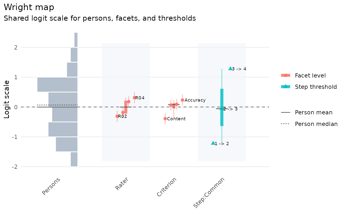
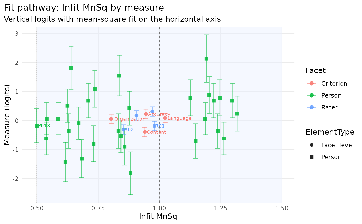
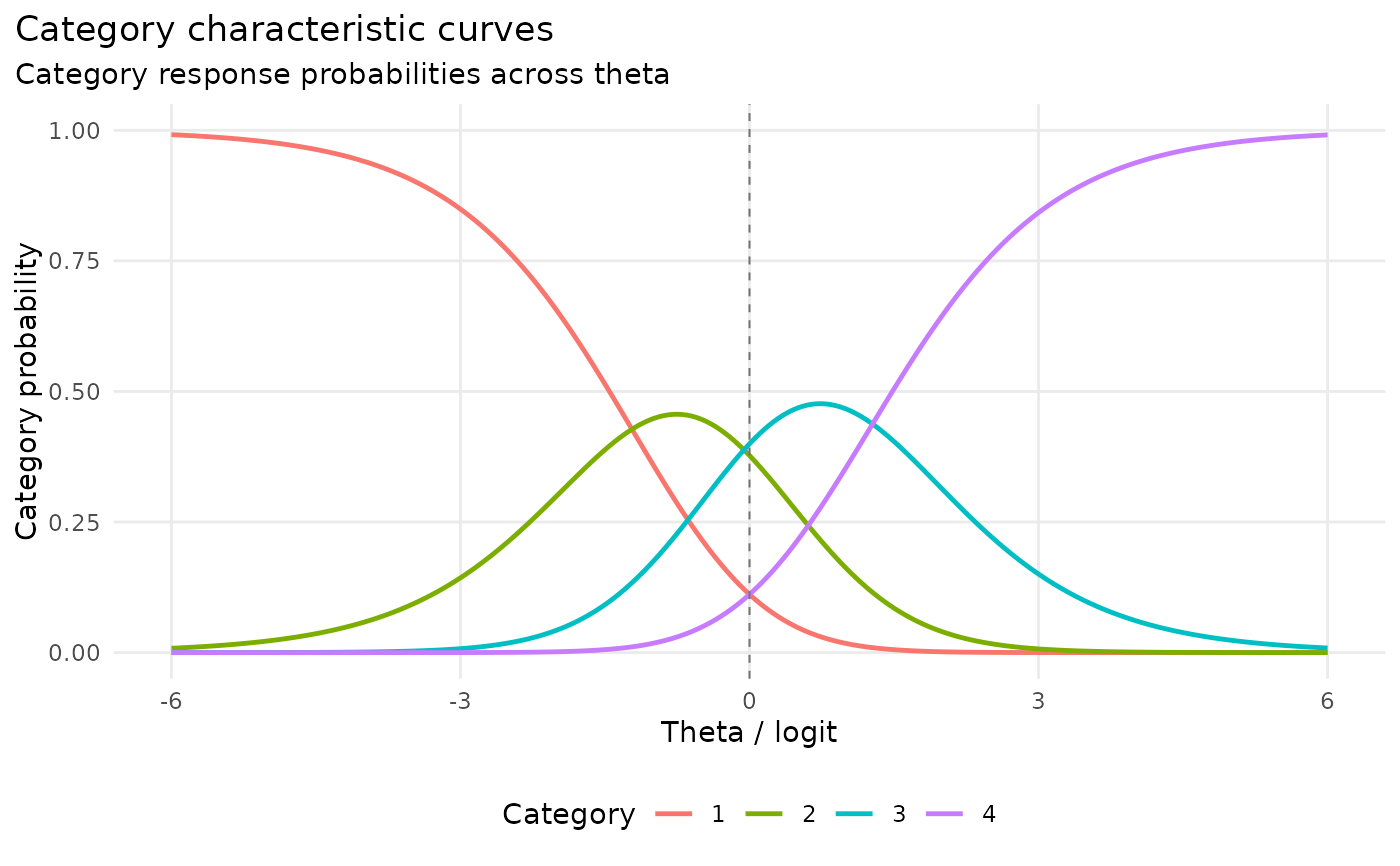
Dedicated conversions are provided for Wright maps, theta-to-expected-score pathways, fit-statistic-to-measure pathways, category characteristic curves, bubble charts, DIF/DFF summaries and heatmaps, portable-calibration score review plots, testlet calibration, shared-rater severity and bootstrap intervals, conditional Person scores, and multivariate D-study comparisons. Matched ordinary/extended facet comparisons preserve centered effects, paired/difference views, excluded rows, display controls and alternative text; see plot.mfrm_extended_comparison(). Threshold-sensitivity tile and curve payloads also preserve their selected view, display controls and text alternatives; see plot.mfrm_screening_sensitivity(). Response residual displays preserve their posterior or conditional plug-in probability definition and lack of reference cutoffs. Paired views retain available Infit when Outfit is undefined; see plot.mfrm_response_diagnostics(). Testlet conversions retain unavailable rows, prior-only symbols and the conditional-interval note; they do not estimate diagnostics or add calibration uncertainty. Extended-model interval, precision and empirical-distribution views preserve display settings, data exclusions and text alternatives; see plot.mfrm_testlet_scores(). Bootstrap conversion retains infinite endpoints as arrows and ordinary intervals as a dashed comparison. D-study conversions preserve G/Phi or SEM panels, fixed-count groups, score units, and unavailable estimates. They do not refit the model or add confidence intervals. For multivariate D-study plots, an explicit component = "series" keeps this dedicated conversion; use plot_data() for other tables. Difference-interval plots from mfrm_multivariate_d_compare() use their base plot() method or plot_data(); automatic conversion is not supported. Residual-PCA scree, reference, excess and loadings plots have dedicated conversions with the default or component = "data". They preserve saved eigenvalues, reference cutoffs, signed loadings and display encodings; method identifiers are not inferred as plotted variables. No PCA is recomputed. External-feature PCA scree, scores and loadings views have dedicated conversions. They preserve selected axes, retained-component symbols, saved group colours and shapes, labels and transformation metadata. Scores retain equal axis units; loading coefficients are not correlations. The default and component = "table" use the same complete PCA view. Use ggplot2::labs(title = NULL, subtitle = NULL) to remove headings from the returned ggplot. No PCA or clustering is refitted. External-feature dendrogram conversion retains the stored merges, heights, leaf order and group boxes, including tied-height cuts. The default and component = "tree" use the same complete view. Labels follow the saved setting; no tree is refitted or partition selected. Source metadata remain available with plot_data(). Heights are not significance or branch support. Imputation co-membership heatmaps have dedicated conversion with the default or component = "matrix". Values retain their all-imputation denominator, selected ID order and fixed zero-to-one scale. Unavailable cells use grey fill and crosses; zero is a valid fraction. The saved legend, labels and imputation count are reused, without recomputing or pooling partitions. Silhouette conversion preserves widths on a fixed minus-one-to-one scale, their saved order and overall-mean line. Numeric profiles preserve original-unit means, medians and counts, using separate symbols with slight vertical offsets. Categorical profiles preserve the category order, unused levels, group counts and within-group proportions on a zero-to-one scale. The default and component = "table" keep the full selected view; categorical profiles also accept component = "matrix". These summaries do not estimate uncertainty, rater quality or sampling stability. For main-effects mfrm_d_study results, use the base plot() method or plot_data() for custom graphics; automatic conversion is refused because generic column selection does not preserve those design comparisons. Pooled fixed-facet MI intervals have dedicated conversion with the default or component = "table". Saved t-interval endpoints, degrees of freedom, contrasts and complete-data information cautions are retained, with no repooling or interval recalculation. Open diamonds mark fixed targets without intervals, crosses mark missing intervals, and arrows mark infinite bounds. Arrow tips are plotting limits, not replacement finite confidence limits. Selecting component does not enable unsupported conversions: it cannot preserve D-study differences through generic column selection. Use plot_data() to extract the table and specify the axes, intervals and grouping explicitly in custom graphics. Other draw-free payloads use a conservative tabular fallback; inspect plot_data_components() when automatic inference is not appropriate. Titles, subtitles, and captions are wrapped at 72 text columns for ordinary figure widths; missing text is omitted. For narrower exports or custom line breaks, override these labels with ggplot2::labs() on the returned plot. Fit plots created with show_title = FALSE or show_notes = FALSE retain those settings on conversion. To set them when converting a fit directly, pass the flags through .... Interpretation and display notes remain available in attr(plot, "mfrmr_notes"), when present in the source payload. Wright, pathway, and CCC conversions share the fit-family series palette, honour monochrome presets and supplied palette overrides, and preserve line-type or point-shape distinctions. CCC categories retain their source order. When slope_aes = "colour", slopes instead use a continuous viridis scale (a grey gradient in monochrome); categories still have line types.

Fixed-facet RSM/PCM intervals retain the selected covariance method, level, status symbols and optional ordinary comparison. Titles, subtitles, captions, reference lines and legends can be changed through the source plot arguments. Methods use both line types and vertical offsets, including in monochrome.

Examples

# \donttest{
toy <- load_mfrmr_data("example_core")
# A balanced slice retains every Rater and Criterion while running quickly.
toy <- toy[toy$Person %in% unique(toy$Person)[1:12], , drop = FALSE]
fit <- fit_mfrm(toy, "Person",
                c("Rater", "Criterion"), "Score", maxit = 30)
as_ggplot(fit, type = "wright")

as_ggplot(fit, type = "fit_pathway", include_person = TRUE)

as_ggplot(plot(fit, type = "ccc", draw = FALSE))

# }