Fit many-facet ordered-response models with a flexible number of facets

Estimate person abilities while accounting for rater severity and other influences on scores, such as criterion difficulty. A facet is one such source of variation; its levels are the individual raters or criteria. Each data row is one rating. Supply its column names with person, facets, and score, as in the complete example below. The default is method = "MML" (marginal maximum likelihood). The RSM / PCM branches are the package's many-facet Rasch-family reference route. GPCM adds positive, level-specific discriminations to one facet. MML permits a different facet to supply category steps; JML requires the same facet for both roles. See "GPCM model and inference" below for the current limits on uncertainty and comparisons. In the example, toy stores the data and fit stores the fitted model. Quoted column names such as "Person" must match the data, including case. For your own CSV, see the "Use your own CSV" section of vignette("mfrmr-workflow", package = "mfrmr"). If the vignette is not installed, mfrmr_workflow_methods and describe_mfrm_data() explain the input checks. Pass the reviewed rating data frame to data, not the object returned by describe_mfrm_data(). Before adapting the example, read "Check defaults before adapting an example" in mfrmr_workflow_methods. The score ladder, missing-row handling and population distribution are analysis choices even when arguments are omitted.

Usage

fit_mfrm(
  data,
  person,
  facets,
  score,
  rating_min = NULL,
  rating_max = NULL,
  weight = NULL,
  keep_original = FALSE,
  missing_codes = NULL,
  model = c("RSM", "PCM", "GPCM"),
  method = c("MML", "JML", "JMLE"),
  step_facet = NULL,
  slope_facet = NULL,
  facet_interactions = NULL,
  min_obs_per_interaction = 10,
  interaction_policy = c("warn", "error", "silent"),
  anchors = NULL,
  group_anchors = NULL,
  noncenter_facet = "Person",
  dummy_facets = NULL,
  positive_facets = NULL,
  anchor_policy = c("warn", "error", "silent"),
  min_common_anchors = 5L,
  min_obs_per_element = 30,
  min_obs_per_category = 10,
  quad_points = 31,
  maxit = 400,
  reltol = 1e-09,
  optimizer = c("auto", "BFGS", "L-BFGS-B"),
  mml_engine = c("direct", "em", "hybrid"),
  population_formula = NULL,
  person_data = NULL,
  person_id = NULL,
  population_policy = c("error", "omit"),
  facet_shrinkage = c("none", "empirical_bayes", "laplace"),
  facet_prior_sd = NULL,
  shrink_person = FALSE,
  attach_diagnostics = FALSE,
  checkpoint = NULL,
  gpcm_mml_identification = c("free_population", "fixed_standard_normal"),
  mml_integration = c("fixed", "adaptive"),
  category_policy = NULL,
  em_score_tol = NULL,
  jml_correction_order = NULL,
  jml_correction_sampling = c("fixed_rosters", "random_rosters"),
  gpcm_mml_start = NULL
)

Arguments

data

A data.frame in long format with one row per observed rating event.

person

Column name for the person (character scalar).

facets

Character vector of facet column names.

score

Column name for the observed ordered category score. Values must be coercible to numeric integer category codes. Fractional values are rejected. Binary 0/1 or 1/2 responses are supported as the ordered two-category special case. When keep_original = FALSE, unused intermediate categories are collapsed to a contiguous internal scale and the mapping is recorded in fit$prep$score_map. If rating_min / rating_max are supplied and the observed scores are a contiguous subset of that range (for example a 1-5 scale with only 2-5 observed), the supplied full range is retained so zero-count boundary categories remain visible in the data-support review. A zero-count boundary category is retained as review evidence. With keep_original = TRUE, however, an unobserved internal category in a polytomous fitted ladder creates an unsupported adjacent-step contrast and fitting stops before optimization with a structured category-support error.

rating_min

Optional minimum category value. Supply this with rating_max when the intended score scale includes unobserved boundary categories.

rating_max

Optional maximum category value. Supply this with rating_min when the intended score scale includes unobserved boundary categories.

weight

Optional weight column name.

keep_original

Logical. FALSE (the current default) collapses non-consecutive observed categories to a contiguous internal scale and records the mapping in fit$prep$score_map (the downstream Count = 0 rows are consequently absent). TRUE preserves the declared scale so unused intermediate categories remain visible in rating_scale_table() and APA outputs, which is recommended for preserving the rubric. This changes which category steps are fitted, not just their displayed labels. Fitting stops if a retained internal category has no observations; reviewing or revising that ladder is a substantive decision, not a formatting option. Retained for compatibility; category_policy = "preserve" or "collapse" makes the choice explicit in new code.

missing_codes

Optional pre-processing step that converts sentinel missing-code values to NA before any downstream logic. One of:

• NULL (default): no recoding; strictly backward-compatible.

• TRUE or "default": FACETS / SPSS / SAS convention set ("99", "999", "-1", "N", "NA", "n/a", ".", "") on the score column only. Person and facet identifiers are preserved because short codes such as "N" can be legitimate labels.

• Character vector: an explicit code set, e.g. c("99", "999", ".a"), applied across the person, facet, and score columns.

Replacement counts are recorded in fit$prep$missing_recoding and surfaced by build_mfrm_manifest(). Equivalent to calling recode_missing_codes() manually before the fit.

model

"RSM" (default), "PCM", or "GPCM".

method

"MML" (default) or "JML". "JMLE" is accepted as a backward-compatible alias for the same joint-maximum-likelihood path.

step_facet

Facet whose levels receive separate step parameters in PCM and GPCM. Supply it explicitly for a final analysis. If it is omitted for PCM, mfrmr uses a unique item-like facet name (for example, Item, Task, or Criterion) when available; otherwise it retains the first-facet fallback with a warning. GPCM always requires an explicit value. This argument is not used by RSM, which has one shared set of rating-scale thresholds.

slope_facet

Slope facet for the GPCM branch. mfrmr estimates one positive slope for every level of this designated facet. Thus slope_facet = "Criterion" gives criterion-specific slopes, whereas slope_facet = "Rater" gives rater-specific slopes. For one slope family, MML allows a distinct step_facet; JML requires slope_facet == step_facet. Criterion and rater slope blocks can also be estimated together with an ordered pair of column names; see "Two slope families" below for the explicit MML contract. With one family, slopes are identified on the log scale with their geometric mean fixed to 1, so the table reports relative discrimination across the selected facet's levels rather than unrelated absolute weights.

facet_interactions

Optional confirmatory two-way interaction terms between non-person facets, supplied as explicit character terms such as "Rater:Criterion" or as a list of length-two character vectors. These interactions are estimated simultaneously as fixed effects in RSM and PCM fits. Person-involving interactions, higher-order interactions, and random-effect interaction terms are outside the current scope.

min_obs_per_interaction

Minimum weighted observations recommended for each interaction cell. Cells below this value are flagged in interaction_effect_table() and handled according to interaction_policy.

interaction_policy

How to handle sparse interaction cells: "warn" (default), "error", or "silent".

anchors

Optional direct-anchor table with facet, level, and fixed logit value columns. Each retained row is a computational equality constraint; it is not merely a declaration that an element is common.

group_anchors

Optional group-mean constraint table with facet, level, group, and target-value columns. Its use requires a defensible external assumption about the group target; it does not create observed overlap.

noncenter_facet

One facet to leave non-centered.

dummy_facets

Facets to fix at zero.

positive_facets

Facets with positive orientation.

anchor_policy

How to handle anchor-review issues: "warn" (default), "error", or "silent".

min_common_anchors

Minimum directly anchored levels per non-Person facet used in the package's local count recommendation. This does not verify cross-run element identity, invariance, or empirical connectedness.

min_obs_per_element

Minimum weighted observations per facet level used in anchor-review recommendations.

min_obs_per_category

Minimum weighted observations per score category used in anchor-review recommendations.

quad_points

Integer number of Gauss-Hermite quadrature points used for MML integration over the person distribution. The default is 31. Useful accuracy/runtime settings are:

7	lightweight screening run; information-criterion deltas, weights, preferences, and LRT are disabled. Helpers such as predict_mfrm_population() and reference_case_benchmark() use this value.
15	intermediate review run when runtime matters; automatic model ranking remains disabled.
31	package default and a starting grid, not evidence by itself that numerical integration is adequate.
61+	user-selected denser grids for same-data sensitivity review; no single order is adequate for every response pattern.

Quadrature adequacy depends on the fitted distribution and score support. Orders whose weights cannot all be represented as positive finite doubles produce an error; increasing the order indefinitely is not supported. Use mml_quadrature_sensitivity() to compare the same model and data on user-selected grids before portable calibration and whenever numerical movement could affect a consequential result. The helper reports continuous differences without choosing a cutoff. Raw AIC/BIC/SABIC remain visible below 31 points for diagnosis, but compare_mfrm() fails closed rather than turning a screening/review grid into automatic selection.

maxit

Computational ceiling on optimizer iterations. The default is 400; for two-family EM this counts outer EM iterations. Two-family adaptive initialization also allows this many EM seed iterations; it then applies separately to every direct optimizer stage at each start. For corrected JML it applies separately to each recorded root-solving stage. This is not a convergence criterion or a model-selection control: a fit that reaches the ceiling remains non-ready until the common convergence and terminal-gradient checks pass. Smaller values used in brief examples are for demonstration only and should not be copied into a substantive analysis without an explicit computational protocol.

reltol

Portable tolerance setting for the initial optimizer stage. For two-family fixed-grid EM, omit this argument and use em_score_tol. Adaptive two-family direct MML uses reltol and the direct optimizer's gradient check. The default is 1e-9. For BFGS this is passed as reltol; for L-BFGS-B it is mapped to factr and pgtol, whose actual values are recorded in the fit. When this setting is at least as strict as the public default (reltol <= 1e-9), optimizer code zero followed by a failed common terminal-gradient review triggers a bounded warm-started polish ladder. The best non-worsening stage under the recorded selection rule is retained. Requested and selected-stage settings remain in fit$summary, and the complete stage history remains in fit$opt$optimizer_polish. If ordinary polishing still stalls, fixed-grid RSM/PCM or adaptive GPCM MML fits with a fixed population and at most 64 free parameters can use one local curvature step to restart the selected optimizer. The step requires positive-definite, well-conditioned curvature, a smaller gradient and an objective that does not worsen beyond floating-point roundoff. The original convergence and terminal-gradient criteria still apply; failed proposals retain their reasons in the stage history. Fixed-grid GPCM MML fits with at most 64 free parameters also check numerical curvature after optimizer code zero. Negative curvature can trigger up to three BFGS restarts in rescaled search coordinates, even when the raw gradient is small. Each restart uses the requested maxit ceiling. A replacement must pass the original gradient/convergence checks, have no detected negative curvature and not worsen the objective beyond roundoff. Failed recovery retains the estimate with a numerical warning. This changes only the search coordinates, not the model or information matrix used for inference. It does not establish a global optimum, adequate quadrature, or valid confidence intervals. Inspect the SmallestCurvature, CurvatureScale and CurvatureReviewError fields in the stage history alongside the objective and terminal gradient.

optimizer

Direct-optimization method. "auto" (default) uses the BFGS M step for the two-family EM route. For other routes it uses the limited-memory "L-BFGS-B" method for MML and for larger JML parameter vectors (at least 200 free parameters), while retaining BFGS for smaller JML fits. Use "BFGS" or "L-BFGS-B" to request one method explicitly. The method actually used is recorded in fit$summary$OptimizerMethod. For L-BFGS-B, inspect OptimizerFactr and OptimizerPgtol rather than interpreting EffectiveReltol as a native stats::optim() control.

mml_engine

MML optimization engine for method = "MML": "direct" (default) uses the selected direct optimizer on the marginal log-likelihood, "em" uses an EM loop for RSM / PCM with population = NULL, or the explicitly scoped two-family GPCM route described below, and "hybrid" uses EM as a warm start before the direct optimizer. Unsupported one-family combinations fall back to "direct" and record that fallback in fit$summary. Direct, hybrid, and EM engines all require the common terminal-gradient check for the Numerical component of fit readiness; EM relative log-likelihood convergence alone does not establish numerical readiness. InferenceReady is TRUE only when every stored fit-readiness component passes.

population_formula

Optional one-sided formula for a person-level latent-regression population model, for example ~ grade + ses. Latent regression is implemented only for method = "MML" with a unidimensional conditional-normal population model. With NULL, RSM/PCM MML uses a fixed \(N(0,1)\) basis; default GPCM MML instead estimates an intercept-only normal population. Version 0.2.4 does not accept arbitrary fixed normal means or standard deviations: portable RSM/PCM calibration and its anchors are defined on the standard-normal basis, and a silent change of basis would change the meaning of those stored values.

person_data

Optional one-row-per-person data.frame holding background variables for population_formula. Numeric, logical, factor, ordered factor, and character predictors are expanded through stats::model.matrix(); categorical xlevels and contrasts are stored for replay and scoring. Prediction-aware transformations such as scale(), poly() and splines::ns() retain their training basis when scoring new persons. Required when population_formula is supplied.

person_id

Optional person-ID column in person_data. Defaults to person when that column exists in person_data.

population_policy

How missing background data are handled for a latent-regression fit. "error" (default) requires complete person-level covariates; "omit" fits the model on the complete-case subset and records omitted persons / omitted response rows in the returned population metadata while retaining the observed-person-aligned pre-omit table for replay/export provenance.

facet_shrinkage

Character. "none" (default) keeps the unshrunk fixed-effects estimates. "empirical_bayes" applies a post-hoc James-Stein / empirical-Bayes shrinkage to each non-person facet (Efron & Morris, 1973); fit$facets$others gains ShrunkEstimate, ShrunkSE, and ShrinkageFactor columns, and fit$shrinkage_report records the per-facet prior variance and effective degrees of freedom. "laplace" is retained as a compatibility alias for "empirical_bayes"; it does not fit a penalized likelihood.

facet_prior_sd

Optional numeric scalar. When supplied, the shrinkage prior variance is fixed at facet_prior_sd^2 instead of being estimated by method of moments. Useful for eliciting a prior from domain knowledge or a previous fit.

shrink_person

Logical. When TRUE and facet_shrinkage is active, the same empirical-Bayes shrinkage is applied to fit$facets$person. Default FALSE, since MML already integrates over a normal population distribution for theta; the option mainly benefits JML.

attach_diagnostics

Logical. When TRUE, diagnose_mfrm() is run once after the fit with residual_pca = "none", and the per-level SE, Infit, Outfit, InfitZSTD, OutfitZSTD, and PtMeaCorr columns from diagnostics$measures are merged onto fit$facets$others (non-person facets) and fit$facets$person (Person rows). This is convenient when downstream code expects a FACETS Table 7 style facet table with fit statistics in one place, and lets summary(fit) show per-person fit columns alongside the measure. For person rows, an existing posterior SE (typical for method = "MML") is preserved and the diagnostic SE is only attached when the existing column is empty. Adds diagnostic runtime (typically +1-2 s on moderate designs) and sets fit$config$attached_diagnostics = TRUE. Default FALSE preserves the minimal Facet / Level / Estimate layout.

checkpoint

Optional list(file = ..., every_iter = ...). When supplied, the MML EM engine writes its state to file every every_iter outer EM iterations using checked same-directory replacement. If the file already exists when the fit starts, the engine resumes only when its versioned identity exactly matches the current data, model, parameter layout, constraints, quadrature, package version, and engine stage. Legacy, corrupt, or incompatible files fail closed. A non-converged pure-EM run may resume with a larger maxit; a completed checkpoint cannot re-enter the same iteration boundary. Only the EM engine (mml_engine = "em" or the EM warm-start step of mml_engine = "hybrid") honours the checkpoint; the direct optim() engine ignores it. Use this to make long MML EM fits crash-resilient on shared compute environments.

gpcm_mml_identification

Scale-identification convention for model = "GPCM" with method = "MML". "free_population" (the default) estimates an intercept-only person distribution \(N(\beta_0,\sigma^2)\) when population_formula is omitted, while retaining geometric-mean-one relative slopes. This restores the common discrimination degree of freedom used by a conventional fixed-latent- variance GPCM; in the documented item-only overlap it is a one-to-one reparameterization of ConQuest scoresfree GPCM. An explicitly supplied population_formula is retained under this convention. With one slope family, "fixed_standard_normal" is the legacy restricted branch: it requires population_formula = NULL, fixes the person distribution to \(N(0,1)\), and also fixes the slope geometric mean to one. The latter is then a substantive relative-discrimination restriction rather than an identification requirement. With two families, fixed N(0,1) instead accompanies a geometric-mean-one first family and free second-family slopes. This argument does not change JML, whose geometric-mean-one slope constraint is required to identify its freely estimated person coordinates.

mml_integration

Numerical integration for MML: "fixed" (default) uses a common Gauss-Hermite grid relative to each person's normal prior; "adaptive" centers and scales the grid at each person's posterior mode on every objective evaluation. Adaptive fitting uses the gradient of the moving-node objective, including changes in its center and width. It requires method = "MML", mml_engine = "direct", and no checkpoint. The choice also controls the fitted likelihood, Hessian, posterior person summaries, fitted-object scoring, and supported portable calibration. quad_points remains the order; neither integration mode guarantees adequate accuracy at a particular order. Compare orders before reporting. During adaptive optimization, trial values that cause numerical overflow are rejected so the search can shorten its step. Starting values must still be evaluable, and final estimates must pass the usual convergence checks; rejecting a trial does not establish a parameter boundary or impose a discrimination upper limit. Adaptive fits with nonlinear coordinates have no completed probability- map identification audit; GPCM also lacks an adaptive slope-boundary audit. These fits remain review-only for formal parameter inference. ConQuest exports currently require fixed integration.

category_policy

Optional explicit category choice: "collapse" maps gaps in the observed categories to consecutive scores; "preserve" keeps the intended ladder, declared with rating_min and rating_max. This changes the fitted category steps, not just labels. NULL (default) uses keep_original, whose default is FALSE ("collapse"). Supplying both choices is allowed only when they agree. Preservation does not estimate unsupported steps: fitting stops if a retained internal category has no observations. Use the same policy in describe_mfrm_data() and review_mfrm_anchors().

em_score_tol

Stopping tolerance for the two-family GPCM MML-EM route only. NULL selects 1e-6 for that route. Stops when the largest absolute derivative of the negative marginal log likelihood, divided by the number of Persons, is at most this value. It does not control interval eligibility. The ascent-checked BFGS M step allows 100 iterations with reltol = 1e-12; both the marginal likelihood and EM auxiliary objective must not decrease beyond numerical roundoff. If BFGS stops before the requested score accuracy, usable positive curvature can refine the auxiliary objective with the same E-step counts. The ascent checks still apply. Dense curvature refinement is limited to 1–64 free parameters; otherwise the ordinary M-step proposal is retained. The saved fit$opt$em_trace records refinement attempts and failures; mstep_score is the proposal's auxiliary-objective score before any step halving. Other model routes require NULL.

jml_correction_order

NULL (default) leaves the usual estimator unchanged. A positive integer explicitly selects an experimental profile-score adjustment for shared-owner model = "GPCM", method = "JML". There is no automatic choice of order. See Corrected JML for the input restrictions, uncertainty meaning and connected outputs.

jml_correction_sampling

Sampling assumption for corrected JML's Person covariance: "fixed_rosters" (default) centers contributions within each observed assignment pattern; "random_rosters" centers globally when assignment patterns are sampled. This changes covariance, not the point equation. The fixed-roster calculation needs at least two Persons per pattern. Both describe new independent Persons, including variation in their ability composition; neither estimates the variance from reassessing the same Persons at fixed abilities. Omit this argument when no correction is requested.

gpcm_mml_start

Initial values for two-family adaptive direct MML only. NULL (default) selects "neutral_em": optimize from both the neutral vector and a same-data fixed-grid EM vector, and select the lowest finite adaptive negative log likelihood, retaining its convergence status. "neutral" retains the earlier neutral-only initialization. Numerical optimizer repairs still apply; exact historical reproduction requires the original source. An EM vector is only a start; its fixed-grid likelihood is never compared with an adaptive likelihood. The seed uses the requested quadrature order, maxit outer iterations, 100 M-step iterations and per-Person score tolerance 1e-6. A finite seed need not have converged. Each direct start uses the requested optimizer, reltol and its existing polishing sequence. All starts, errors, warnings, stage histories, seed trace and elapsed costs are stored in fit$opt$mml_initialization; results and reports include its comparison table. This comparison does not prove a global optimum or interval validity.

Value

An object of class mfrm_fit (named list) with:

• summary: one-row model summary including LogLik, Deviance, canonical free dimension Npar, response-row/weight/Person counts, the versioned information-criterion contract, Person-based MML AIC/BIC/SABIC, explicitly descriptive legacy fields when the common panel is ineligible, and convergence; it also includes user-facing Method, engine-facing MethodUsed, MML-engine fields, terminal-gradient readiness, requested/selected-stage tolerance settings, and the actual L-BFGS-B OptimizerFactr / OptimizerPgtol controls when applicable

• facets$person: person estimates (Estimate; plus SD for MML), with SourceFitReadiness, SourceInferenceReady, and EstimateUse separating a defined Person summary from the source fit's permission to interpret it. In particular, a finite prior-regularized MML EAP does not become reportable when the source fit is blocked.

• facets$others: facet-level estimates for each facet

• steps: estimated threshold/step parameters as a one-row-per-step tibble with Estimate. Bare fits keep this table as point estimates. diagnose_mfrm() exposes MML observed-information step uncertainty in diagnostics$parameter_uncertainty$steps. Check CIEligible and CIUse: finite curvature-based bands alone do not establish ordinary inference. When attach_diagnostics = TRUE, those SE, confidence-limit, and status columns are attached to fit$steps when the Hessian is available. For step-structure quality, also use the step-collapse and disordering warnings from diagnose_mfrm() and category_structure_report().

• slopes: discrimination parameters for GPCM fits as a one-row-per-slope-element tibble. LogEstimate and Estimate retain the finite optimizer values for compatibility and numerical diagnosis; OptimizerLogEstimate / OptimizerEstimate name that role explicitly. Read ParameterStatus, PrimaryLogEstimate, PrimaryEstimate, SEEligible, CIEligible, and ReasonCodes before interpretation. A certified JML slope-only path receives a typed extended-real primary boundary. config$boundary_audit retains the supporting fixed-objective, joint-path, and terminal-gradient records. A certified path can establish that a finite JML maximum is unattained for the evaluated case. The converse is deliberately not used: failure to find a path in the evaluated families, or retention of a finite optimizer point, does not establish existence of a finite global maximum for the non-concave GPCM likelihood. These JML diagnostic records do not supply uncertainty estimates, MML results or evidence of agreement with other software. config$boundary_audit$gpcm_terminal_gradient_stability reconstructs the same fixed JML objective and analytic terminal gradient, checks stored optimizer/polish summaries and deterministic central-difference probes, and reports gradient norms by free-parameter block. Positive boundary certificates take precedence over a finite-point zero or small gradient; otherwise a coherent small gradient is retained-point first-order evidence only. The numerical tolerance is not a statistical significance threshold. These checks do not establish a finite global maximum, boundary absence, uncertainty, external comparability, or readiness. The conditional JML boundary checks are not reused for MML. confint(fit, parm = "slopes") and diagnose_mfrm() separately check the current local MML solution before supplying approximate pointwise relative-slope intervals. CIEligible and InferenceReview record this output-specific decision, without overriding the global boundary audit. Ineligible local calculations remain in Optimizer*SE / Optimizer*CI. Refresh saved fits through either function; no refitting is necessary. The identification convention pins the geometric mean of finite optimizer slopes at 1.

• readiness: the versioned fit record, five component rows, and current parameter-level rows. The current parameter slice includes GPCM slopes; other non-Person parameter classes remain scheduled for later propagation.

• interactions: model-estimated facet interaction effects and metadata when facet_interactions is supplied

• population: population-model metadata. Ordinary RSM/PCM and JML fits keep an inactive record (active = FALSE, posterior_basis = "legacy_mml"). Default GPCM MML and active latent-regression fits store the fitted design matrix, regression coefficients, residual variance, omission review, the complete-case estimation table (person_table), and the observed-person-aligned replay/export provenance table retained before complete-case omission (person_table_replay), plus stored categorical xlevels / contrasts for model-matrix replay and scoring, together with posterior_basis = "population_model". estimation_converged records optimizer convergence and inference_ready records the separate formal readiness decision. The older population$converged field is retained as a compatibility alias of inference_ready; its basis is recorded in population$converged_basis.

• data_review: pre-fit Data, Design, Stability, and Reporting readiness evidence propagated into summaries and plot-interpretation checks

• config: resolved model configuration used for estimation, including config$anchor_review and the recorded estimation controls

• prep: preprocessed data/level metadata

• opt: optimizer result augmented with optimizer_diagnostics, the complete optimizer_polish stage history, method-selection metadata, and evaluation-cache counters. For direct fitting, its core fields originate from stats::optim(); EM additionally records engine-specific diagnostics.

Details

Data must be in long format (one row per observed rating event). Exact duplicate Person-by-facet combinations are retained, warned once, and propagated as a Data review state. They are not treated as independent replication evidence. A legitimate re-rating or replicated scoring event should be represented by an event, occasion, or other distinguishing facet before fitting.

Corrected JML

When each Person has few ratings, ordinary JML can retain structural bias even with many Persons. The explicit jml_correction_order option adjusts the profile-score equation to address this source of bias. It changes the estimator, not the response model. A higher order is not necessarily more accurate: bias, variance and numerical stability can change in different directions. Choose the order as part of the analysis plan and examine sensitivity; neither AIC nor the smallest RootSE chooses a justified order.

This experimental route requires the optional nleqslv package, observed integer scores, declared rating_min and rating_max, additive fixed facets, and a single explicit step_facet that also owns the slopes. Facet names are unrestricted. Use category_policy = "preserve" to retain the declared score ladder. All facet locations and each step ladder sum to zero; slopes have geometric mean one. Persons are independent sampling units, with conditionally independent ratings within Person. Only observed assignments contribute; unassigned or missing scores are not imputed. Repeated cell rows are treated as independent responses, not correlated repeated measurements. Fixed anchors, nonunit weights, interactions, shrinkage, separate slope/step owners, corrected RSM/PCM, and ordinary optimizer controls are unavailable. Explicit unsupported arguments produce an error rather than being ignored.

For an order \(k\), the equation uses \(U_k=(I-K_\beta)^k U_0\), where \(U_0\) is the negative profile-likelihood score and \(K_\beta\) averages over responses at their profiled Person MLE. This is the MLE plug-in construction discussed by Dhaene and Weidner (2023, section 8.1), applied here to the declared GPCM structure. Exact owner-total enumeration is limited to 5,000 joint states per assignment pattern; larger calculations stop explicitly. No approximate pruning is substituted. The full equation Jacobian and empirical Person contributions give a sandwich covariance, with the selected assignment-sampling assumption. This is not an inverse likelihood Hessian or a general proof of bias removal.

For example, "fixed_rosters" describes new cohorts with the same number of Persons assigned to each rater/task combination. It does not hold each Person's ability fixed across repeated cohorts. Ability distributions are unspecified and may differ between assignment patterns. With "random_rosters", both Persons and their assignments are sampled from the same joint population; assignment need not be independent of ability. Neither option models shared random raters or dependent Persons. The empirical sandwich has no small-sample degrees-of-freedom correction. Its fixed-roster interpretation requires enough independent Persons within each pattern; two Persons is a computational minimum, not an assurance of accurate uncertainty. Taking "random_rosters" solely to obtain a RootSE changes the sampling assumption and is not a repair for sparse information.

Use summary(fit)$tables for locations, steps, relative slopes and the uncertainty explanation; include_person = TRUE adds Person profiles. RootSE describes local variation around the adjusted-equation solution, which may remain biased for the true structural parameter. LogRootSE describes log-slope variation. Neither is supplied as a standard error with established structural coverage; no confidence limits are constructed. Persons are reprofiled at the adjusted calibration, with infinite limits for extreme scores and no invented Person SE. Numerical attempts remain available in summary(fit)$attempts and fit$jml_adjustment.

A valid point estimate is retained if covariance is unavailable, with its reason. Different accepted roots yield missing primary estimates rather than selection by the ordinary likelihood. Agreement between starting values is a local check, not proof of a unique global solution. A failure remains a reportable fitted object with missing estimates and its attempts.

plot(fit, type = "slopes"), "locations" (select one facet) and "steps" show point estimates. Choose style = "distribution" for an empirical cumulative view; as_ggplot(plot(fit, draw = FALSE)) is supported. Use mfrm_results(fit) then mfrm_report() or export_mfrm_results() to retain these meanings through reporting and saved replay. For conditional probabilities and descriptive residuals on the observed fitted rows, use mfrm_response_diagnostics() and attach the saved result with mfrm_results(fit, response_diagnostics = result). This holds corrected calibration and Person profiles fixed; no posterior averaging, uncertainty intervals or fit cutoffs are supplied. Extreme-score probabilities remain available; zero variance prevents standardization, with separate availability for Infit and Outfit. See that helper's help before interpreting a summary. For new Persons, predict_mfrm_units() and extract_mfrm_calibration() provide conditional EAP scoring after their corrected-equation source checks. These scores add a separate normal reference prior. Their posterior intervals condition on calibration and do not establish structural coverage or remove residual bias. The portable artifact omits training responses and Person estimates; its own summary and score plots retain the correction order. Ordinary fit tests, Wright/Pathway maps, structural confidence intervals, likelihood ranking and corrected Person ML/WLE remain unavailable. The default MML and uncorrected JML workflows are unchanged.

Two slope families

To estimate, for example, criterion and assessor discrimination together, use slope_facet = c("Criterion", "Assessor"). The order declares roles: the first facet has centered locations and slopes with geometric mean one; the second has free locations/slopes and owns the centered category steps. The product of their slopes multiplies the complete adjacent-category predictor. There is still one ability dimension. Column names and data column order do not select these roles.

This route requires exactly those two non-Person facets, model = "GPCM", method = "MML", gpcm_mml_identification = "fixed_standard_normal", either fixed integration with mml_engine = "em" or mml_integration = "adaptive" with mml_engine = "direct", and both step_facet and noncenter_facet set to the second slope facet. These options must be chosen explicitly; the one-family defaults are not silently replaced. Use observed, unweighted integer scores on a scale from zero to rating_max, without missing IDs, duplicate person-facet rows or surrounding ID whitespace. Categories are not collapsed; if any are absent, declare rating_max and category_policy = "preserve" so category-support checks can assess that scale. Unobserved assignments are not zero scores. Anchors, population covariates, shrinkage, interactions, positive/dummy facets, checkpoints and automatic diagnostics are not supported in this route; explicitly supplying their arguments, including unused policy controls, produces an error. Fixed-grid EM uses em_score_tol; adaptive direct MML uses reltol and the direct optimizer's gradient check. Passing the other engine's tolerance is an error. Adaptive integration preserves the same N(0,1) population and response equation while moving each Person's grid. It is direct maximization of the marginal likelihood, not adaptive EM. By default it compares neutral and EM-derived starts through that same adaptive objective; see gpcm_mml_start. A better unfinished solution is retained as unfinished, rather than replaced by a worse converged candidate. If a retained starting point is better than all terminal candidates beyond roundoff, the returned fit remains numerically unresolved. A failed alternative is disclosed; if every direct attempt fails, the error carries an initialization record. Neither fixed-grid likelihoods nor interval outcomes select a candidate. Extreme slopes and weak information can still prevent inference even after a successful start comparison. Use mml_quadrature_sensitivity() to compare refits at different orders; it preserves the chosen integration method, engine and initialization policy.

summary(fit) and print(fit) retain numerical status and the two slope references. mfrm_curve_intervals() evaluates provisional category or per-rating information curves at supplied abilities; all their intervals are unavailable. Use plot(curves) and mfrm_results(fit, include = c("fit", "plots"), compute = "never", intervals = list(curves = curves)) to report saved curves. Their values can be inspected even after nonconvergence, but are not qualified estimates. Separately request confint(fit) for experimental component log-Wald intervals from the full observed marginal information. Their numerical checks do not qualify global identification or sampling coverage; failed checks retain missing bounds. Attach the result alongside curves for saved plots/reports. For fixed-grid EM, to profile one component instead, explicitly request confint(fit, method = "profile", slope = c(Task = "t1")), replacing the named owner and level with your fitted identifiers. This reoptimizes other coefficients; it is an experimental local interval without established coverage. mfrm_response_diagnostics() integrates each Person's ability posterior at the saved calibration for descriptive residuals. Both slopes are retained; unavailable integration stays explicit. There are no reference fit cutoffs. Attach this result through response_diagnostics in the results call above. Adaptive two-family log-Wald checks use the moving-node marginal objective and compare adaptive quadrature orders. Posterior residuals preserve the fitted integration method and complete conditioning record, with separate row-wise integration checks. Adaptive profile intervals remain unavailable. predict_mfrm_units() separately supplies experimental conditional new-Person EAP and posterior intervals with the retained N(0,1) prior, known levels, unit weights and separate source/batch checks; calibration uncertainty is excluded. mfrm_facet_intervals() separately supplies experimental model-based intervals for either owner's locations and within-facet contrasts, retaining slope/step nuisance uncertainty. Failed numerical checks leave missing bounds; location differences need not imply uniform rating differences. Attach these intervals to mfrm_results() for plots, reports and exports. Step/curve intervals, sandwich inference, model ranking/LRT, ordinary fit/bias diagnostics and Wright/Pathway plots remain unavailable. extract_mfrm_calibration() provides a separately checked portable two-family route. Matching native or portable scores can be attached with mfrm_results(fit, scores = scores) without rescoring. Numerical agreement of the fitting implementation is not a general identification, convergence or coverage guarantee. See vignette("mfrmr-gpcm-scope") for a complete example and interpretation.

Choose the arguments by their purpose

• Identify the ratings: data is the rating table; person, facets and score are quoted column names, not the values in those columns.

• Declare the rubric: set rating_min, rating_max and category_policy consistently with describe_mfrm_data(). The default can collapse gaps; preservation can reveal an unsupported category step.

• Choose the statistical model: model, step_facet, slope_facet, anchors and population arguments determine what is estimated. Ordinary RSM/PCM MML with population_formula = NULL fixes N(0,1); the default GPCM MML instead estimates the normal population mean and variance.

• Control computation: quad_points, maxit, reltol, optimizer and mml_engine govern numerical fitting. Increasing them does not change the model's support or automatically justify statistical inference.

• Choose follow-up output: attach_diagnostics = TRUE computes and attaches diagnostics; the default leaves that separate. summary(fit) explains the result's status; diagnose_mfrm() reviews response fit.

GPCM model and inference

One selected facet supplies level-specific positive discriminations. With MML, a different facet may supply category steps. For example, slope_facet = "Criterion", step_facet = "Rater" estimates a relative discrimination for each criterion and category-step contrasts for each rater. It does not simultaneously estimate rater discriminations. JML requires the same owner for both blocks. The model has one substantive ability dimension; its structural choices and currently unavailable inferential outputs are separate considerations.

Free-slope fits retain numerical estimates for review. confint.mfrm_fit() supplies approximate relative-slope intervals for eligible MML solutions. MML information-criterion ranking uses separate likelihood and local-solution checks in compare_mfrm(). compare_mfrm() and build_weighting_review() also accept nested = TRUE for an equal-slope PCM/GPCM test after verifying matching population and constraint settings. Fitted-object scoring and information have their own scope and do not imply a portable GPCM calibration artifact. Consult gpcm_capability_matrix() for each operation before using its output.

Model

fit_mfrm() estimates many-facet ordered-response models. The RSM and PCM branches follow the many-facet Rasch-family tradition (Linacre, 1989); the GPCM branch extends the partial-credit kernel with estimated positive slopes under the package's documented identification constraints. For the equal-slope RSM/PCM branch, a two-facet design (rater \(j\), criterion \(i\)) is:

$$\ln\frac{P(X_{nij} = k)}{P(X_{nij} = k-1)} = \theta_n - \delta_j - \beta_i - \tau_k$$

where \(\theta_n\) is person ability, \(\delta_j\) rater severity, \(\beta_i\) criterion difficulty, and \(\tau_k\) the \(k\)-th Rasch-Andrich threshold. Any number of facets may be specified via the facets argument; each enters as an additive term in the linear predictor \(\eta\).

With model = "RSM", thresholds \(\tau_k\) are shared across all levels of all facets. With model = "PCM", each level of step_facet receives its own threshold vector \(\tau_{i,k}\) on the package's shared observed score scale.

One response-model family is used per fit_mfrm() call. The current public interface does not combine binary, RSM, PCM, or GPCM observations in one fit, define multiple independent rating scales, or accept general threshold/scale anchors and fixed-calibration starting values.

With model = "GPCM", the adjacent-category kernel is multiplied by a positive slope for the designated slope-facet level:

$$\ln\frac{P(X_{nij} = k)}{P(X_{nij} = k-1)} = \alpha_g(\eta - \tau_{h,k}),\quad \alpha_g > 0.$$

Here \(g\) indexes the slope facet and \(h\) the step facet; MML permits these to differ. Slopes have a sum-to-zero constraint on log slopes, so their geometric mean is 1. Step contrasts are centered within each step owner, separately from facet location effects. Crossing the facets and observing enough categories is necessary to distinguish their effects; allowing separate owners does not ensure identification in a given design. A selected facet owns a vector rather than one common number: if there are \(G\) levels, the fit returns \(G\) positive slopes with \(G-1\) free log-slope contrasts. Every other facet remains additive inside \(\eta\) and receives no separate slope. Selecting a rater facet is therefore a different restricted model from selecting a criterion or task facet. The placement of the slope is part of the model identity: it multiplies the complete adjacent-category predictor, including the person coordinate, all additive facet locations and fitted facet interactions inside \(\eta\), and the owned step. It is not a loading-only formulation in which the slope multiplies ability while rater severity and other intercept terms remain unscaled. Such a formulation, including TAM multifacet GPCM.design constructions with separate linear intercept and slope designs, is a different model unless an algebraic reduction establishes equivalence. In this one-family many-facet GPCM, exactly one facet supplies slopes. MML permits a different step owner; JML requires a shared owner. It is not the broader Uto–Ueno generalized MFRM, whose task and rater slopes enter multiplicatively and whose step owner must be stated separately. The provisional two-family route above fits that product equation with its own scale and output restrictions. Setting every slope to one recovers the equal-discrimination PCM kernel; neither route supplies multidimensional traits or response-style parameters. Under the default one-family gpcm_mml_identification = "free_population" branch, the population standard deviation carries the common discrimination scale while the geometric-mean-one slopes describe relative discrimination. Equivalently, on a standardized latent variable the absolute slopes are \(\sigma\alpha_g\). Under gpcm_mml_identification = "fixed_standard_normal", both the population standard deviation and slope geometric mean are fixed to one; that legacy branch is a narrower relative-discrimination model. Under JML, the geometric-mean-one constraint is required to resolve the ability/slope scale because person coordinates are estimated jointly.

The model name does not imply finite parameter bounds. The JML branch maximizes the identified joint log-likelihood without a statistical penalty or finite bounds on person, location, step, or slope coordinates. Numerical line-search rejection of non-representable slope proposals is not regularization. When a recession direction is certified, the finite optimizer iterate remains a numerical trace and the primary result uses the appropriate extended-real or typed boundary status; it is not relabelled as a finite maximizer of the original JML objective.

With only two ordered categories (\(K = 1\)), the RSM/PCM branch reduces to the usual binary Rasch logit for the single category boundary:

$$\ln\frac{P(X_{n\cdot} = 1)}{P(X_{n\cdot} = 0)} = \eta - \tau_1$$

GPCM uses the slope-scaled counterpart \(\alpha_g(\eta - \tau_{g,1})\).

With method = "MML", person parameters are integrated out using Gauss-Hermite quadrature and EAP estimates are computed post-hoc. With method = "JML", all parameters are estimated jointly as fixed effects. "JMLE" remains an accepted compatibility alias, but package output now uses "JML" as the public label. See the "Estimation methods" section of mfrmr-package for details.

Weighting policy

mfrmr treats RSM / PCM as the equal-weighting reference route for operational many-facet measurement. In that Rasch-family branch, discrimination is fixed, so the scoring model does not differentially reweight item-facet combinations through estimated slopes.

GPCM is supported as an alternative when users explicitly accept discrimination-based reweighting. This often improves model fit, but the package does not treat better fit alone as a sufficient reason to replace an equal-weighting Rasch-family model.

The weight argument is separate from that modeling choice. It supplies an observation-weight column; it does not create a free-form facet-weighting scheme and does not change the fixed-discrimination contract of RSM / PCM.

Input requirements

Minimum required columns are:

• person identifier (person)

• one or more facet identifiers (facets)

• observed score (score)

Scores are treated as ordered categories. Although the fitted category probabilities form a multinomial probability vector, category order is part of the likelihood: unordered nominal/multinomial-logit responses are not supported. Poisson, negative-binomial, and grouped binomial-trial counts are also not response families in fit_mfrm(). Integer counts supplied as score are interpreted only as ordered category codes. Non-numeric score labels are dropped with a warning after coercion, whereas fractional numeric scores are rejected with an error instead of being silently truncated.

A positive numeric weight may encode a replication/likelihood weight for an ordered-rating row when weighting that conditional contribution is the intended estimand. It is not a general collapsed-person frequency-table interface: under MML, powering responses inside one Person's conditional pattern is not the same as replicating a complete Person pattern after marginalization. A weight also does not turn the score into a count outcome or model dependence among repeated ratings. Non-positive finite weights are excluded during preparation, and non-unit observation-weight fits are not eligible for ordinary inference, facet equivalence, or the common MML information-criterion panel under the current package contract. Normalizing weights to mean one does not remove this restriction. Point estimates and computed curvature/posterior precision remain available for diagnostic review; they do not establish sampling SEs or confidence coverage for the weighted objective. Omitted weights and explicitly all-unit weights use the same eligibility rules. Earlier saved fits require refitting or a current readiness audit; their old inference flags are not carried forward.

The fitted many-facet ordered-response model assumes conditional independence of observations given the person and facet parameters (Linacre, 1989). Repeated ratings of the same person-criterion combination by the same rater violate this assumption. When such structures may be present, follow fitting with diagnose_mfrm(fit, diagnostic_mode = "both"); its strict_pairwise_local_dependence screen is an exploratory check for residual dependence beyond what the additive linear predictor absorbs.

Binary responses are therefore supported as ordered two-category scores (for example 0/1 or 1/2) under the same ordered-response interface. If your observed categories do not start at 0, set rating_min/rating_max explicitly to avoid unintended recoding assumptions. For example, if the intended instrument is a 1-5 scale but the current sample only uses 2-5, set rating_min = 1, rating_max = 5 to retain the zero-count category 1 in the data-support review. That boundary absence is a review condition for the separate element-boundary contract, not by itself an unsupported free step contrast. By contrast, retaining an unobserved internal category in a polytomous fitted ladder creates an adjacent-step recession direction, so fit_mfrm() stops before optimization rather than reporting finite step estimates for that ladder. If these bounds are omitted, the observed score range is used and the provenance is stored in fit$prep and summary(fit)$settings_overview. Set options(mfrmr.show_inferred_rating_range = TRUE) when you want an interactive reminder whenever a bound is inferred. Data-preparation events such as row drops, ID trimming, duplicate person-by-facet cells, and single-level facets are stored in fit$prep$row_retention and fit$prep$preparation_notes. Routine row-drop/trim/single-level messages are quiet by default; set options(mfrmr.show_preparation_messages = TRUE) to show them during interactive checks.

When keep_original = FALSE, observed gaps such as 1, 3, 5 are recoded internally to a contiguous scale (1, 2, 3) and the mapping is stored in fit$prep$score_map. To retain zero-count intermediate categories as part of the original scale, set keep_original = TRUE in addition to supplying the full rating_min / rating_max range.

Fixed effects assumption (facets have no prior)

fit_mfrm() follows the Linacre (1989) many-facet Rasch specification: person ability is integrated out under a N(0, 1) distribution (or under the N(X\beta, \sigma^2) population model when population_formula is supplied). GPCM MML instead activates an intercept-only N(\beta_0, \sigma^2) population model by default so its common discrimination scale is estimable. Every facet parameter (Rater, Criterion, Task, ...) is estimated as a fixed effect identified by a sum-to-zero constraint. There is no hierarchical prior, no shrinkage, and no variance component for the facets.

Practical implication: when a facet has very few observed levels (for example 3 raters) or some of its levels have very few ratings (for example 5 ratings per rater), the fixed-effect estimates retain wide SEs, and extreme estimates are not pulled toward the facet mean. Jones and Wind (2018) note that rater estimates in particular are "more sensitive to link reductions" than examinee or task estimates. For a publication-workflow review of this, use:

• facet_small_sample_review() for per-level N and SE bands against Linacre (1994) sample-size guidelines.

• detect_facet_nesting() and analyze_hierarchical_structure() when raters are nested in regions, schools, or other strata that the additive fixed-effects MFRM cannot partition out.

• compute_facet_icc() and compute_facet_design_effect() for descriptive variance- component summaries based on lme4 (optional).

fit$summary$FacetSampleSizeFlag summarizes the worst Linacre band across non-person facet levels ("sparse" < 10, "marginal" < 30, "standard" < 50, "strong" >= 50).

Estimator choice and the JML incidental-parameter caveat

Joint maximum likelihood (method = "JML" / "JMLE") estimates both the structural parameters (facets, thresholds, slopes) and every person measure as fixed parameters in one optimization. This is the incidental-parameter problem of Neyman & Scott (1948): structural-parameter bias can persist as the number of persons grows with the number of items per person held fixed. In classical Rasch settings this bias can be of order \(1/L\) (where \(L\) is the number of items per person) and therefore need not vanish by adding persons alone. Wright & Stone (1979) and Wright & Masters (1982, ch. 5) document an empirical \((L-1)/L\) correction that approximately removes the bias for the dichotomous Rasch model; mfrmr does not apply that correction (no bias_correction argument exists). A common positive multiplier is not a correction for relative GPCM slopes: multiplying all slopes by the same factor leaves their ratios unchanged, and rescaling them to geometric mean one returns the original slopes. A correction for relative slopes therefore needs its own justification.

Uncorrected JML facet/location SEs use observation-table information: $$\mathrm{SE}_{g} \approx \left[\sum_{r \in g} w_r a_r^2 \mathrm{Var}(X_r \mid \widehat\eta_r)\right]^{-1/2}.$$ Here \(g\) is a facet level, \(r\) an observed response row, \(w_r\) its weight, and \(a_r\) its GPCM slope (one for RSM/PCM). Only finite information contributions are used. These exploratory SEs treat the other fitted parameters as fixed; they are not slope SEs or a joint covariance adjusted for estimating Person and structural parameters together. The local joint-curvature check used for portable GPCM JML scoring does not supply such an inferential covariance. Values fixed by anchors or identification constraints are not estimated: diagnostic tables mark them Fixed = TRUE and leave their sampling SEs and intervals missing, rather than assigning an observation-information SE.

Nuisance-parameter adjustment and estimation bias are separate issues. Haberman (2004, Sections 1.4-1.5) shows for a binary Rasch setting that, with fixed test length, JML can concentrate around a biased limit as the number of persons grows. Even a variance appropriate to that limit does not establish coverage of the true parameter. This result motivates checking test length separately from sample size; it does not validate a correction or an interval for sparse many-facet GPCM. Formal JML slope intervals are not currently available in mfrmr.

When comparing software, report response-score adjustment and post-fit bias correction separately, including how the correction defines exposure when responses are missing or unequal across Persons. Matching the label "JML" alone does not establish matching estimates or uncertainty.

Practical recommendation:

• For manuscript or operational reporting, choose the estimator from the inferential target and assumptions, and report the choice. MML integrates person measures under a specified population model and provides marginal observed-information SEs; consistency of its structural estimates is conditional on an adequate response model, population distribution, and regularity conditions.

• JML remains useful for a JMLE-oriented FACETS comparison, descriptive or exploratory work, and designs with substantial information per person. Report its incidental-parameter limitation and the exploratory basis of this package's JML structural SEs rather than treating estimator choice as a universal reporting rule.

• For supported Rasch-family formulations, conditional maximum likelihood is a distribution-free alternative that conditions out person parameters. A third-party CML fit can be imported from eRm with import_erm_fit().

All-minimum and all-maximum Persons

fit_mfrm() has no public option to remove Persons before fitting because all their responses are at the minimum or maximum. Both JML and MML retain those observed responses. Extreme-response flags use the usable rows after data preparation; missing responses do not count as intermediate scores. Declare rating_min and rating_max from the rubric so that an observed maximum is not mistaken for the intended scale maximum. Inspect fit$facets$person$Extreme for "low", "high", or "none".

Ordinary JML. fit_mfrm() does not replace extreme response scores before JML fitting. For an independently free Person with all-minimum or all-maximum responses, the primary Estimate is -Inf or Inf; OptimizerEstimate retains the finite computational trace, not a finite Person MLE. Fixed Person anchors retain their supplied values, and coupled constraints require their own boundary review. The Person audit's BoundaryState = "has_exclusions" identifies nonfinite parameters; it does not mean that these Persons or their input rows were deleted. Finite structural estimates alone do not establish a finite joint maximum.

Corrected JML. In the supported shared-owner GPCM route, extreme Persons also remain in the data and assignment-pattern accounting. Their profiled abilities have infinite limits and their structural estimating- equation contributions are zero at those limits. This boundary calculation is not an input filter or a general proof of bias removal.

MML. Extreme Persons contribute to the marginal likelihood through integration over the specified or estimated population distribution. Their reported abilities are posterior EAPs, with posterior SDs rather than frequentist Person-MLE standard errors. A proper normal population model with finite parameters gives finite EAPs, subject to valid numerical integration; an extreme response pattern alone does not require deletion. This does not guarantee convergence, identification or valid structural intervals for the fitted model. Removing these Persons would change the observed sample and marginal likelihood.

New-Person scoring with predict_mfrm_units() is a separate operation. With an eligible calibration and an admitted scoring prior, it can return finite EAPs for extreme new Persons, including after JML calibration. Those scores do not replace the original JML Person MLEs. Calibration-source checks and scoring-batch integration checks must both pass; increasing scoring nodes does not resolve a boundary in the source calibration. A finite display from fair_average_table(..., xtreme = ...), or placement at the end of a Wright map, likewise does not change the fitted model or correct JML bias.

Model-estimated facet interactions

facet_interactions adds confirmatory fixed-effect interaction terms to the linear predictor. For example, facet_interactions = "Rater:Criterion" estimates a rater-by-criterion deviation matrix in the same likelihood as the main MFRM fit. The additive reference is

$$\eta_{nij} = \theta_n - \delta_j - \beta_i$$

and the interaction extension is

$$\eta_{nij} = \theta_n - \delta_j - \beta_i + \gamma_{ji}$$

where the interaction block is identified by zero marginal sums:

$$\sum_j \gamma_{ji} = 0,\quad \sum_i \gamma_{ji} = 0.$$

With \(J\) levels of the first facet and \(I\) levels of the second facet, this contributes \((J - 1)(I - 1)\) free parameters. Positive interaction estimates indicate scores higher than expected under the additive main-effects model for that facet-level combination; negative estimates indicate lower-than-expected scores.

This is a model-estimated interaction term, not the residual screening reported by estimate_bias() or estimate_all_bias(). In line with the MFRM bias-interaction literature, the facet pair should be named explicitly before fitting. Exploratory use is possible, but should be reported as screening, with sparse-cell and multiplicity caveats. The current implementation is intentionally narrow: two-way non-person facet interactions for RSM and PCM only, estimated as fixed effects. GPCM interactions, person interactions, higher-order interactions, and random-effect facet interactions are deferred.

This is ordered binary support, not a separate nominal-response model. In PCM, a binary fit still uses one threshold per step_facet level on the shared observed-score scale.

Supported model/estimation combinations:

• model = "RSM" with method = "MML" or "JML"/"JMLE"

• model = "PCM" with a designated step_facet (defaults to first facet)

• facet_interactions with model = "RSM" or "PCM" for explicit two-way non-person facet interactions

• model = "GPCM" uses one positive slope family. MML permits separate slope/step owners; JML requires slope_facet == step_facet. Core summaries, fitted-object posterior scoring, compute_information(), Wright/pathway/CCC fit plots, diagnose_mfrm(), residual-PCA follow-up, interrater_agreement_table(), unexpected_response_table(), displacement_table(), measurable_summary_table(), rating_scale_table(), facet_quality_dashboard(), reporting_checklist(), category_structure_report(), category_curves_report(), and graph/scorefile facets_output_file_bundle() routes are available with score-side caveats. Separate-owner MML supports slope and curve intervals, same-design bootstrap_mfrm_gpcm(), and matched PCM comparison. build_weighting_review() and the following simulation/design workflows still require the same slope/step owner. Direct simulation specifications and data generation are also supported through build_mfrm_sim_spec(), extract_mfrm_sim_spec(), and simulate_mfrm_data() when the slope-aware generator contract is stored explicitly; direct recovery checks are available through evaluate_mfrm_recovery() and assess_mfrm_recovery(). Slope-aware fair_average_table() and estimate_bias() are available with their documented caveats. Role-based design evaluation, population forecasting, diagnostic-screening, and signal-detection helpers are available as caveated sensitivity evidence. Full FACETS-style score-side contract review, posterior predictive checks, and MCMC estimation are not available for GPCM. Use gpcm_capability_matrix() as the formal boundary statement for the current GPCM scope.

Latent-regression status:

• population_formula = NULL keeps the standard unconditional behavior for RSM/PCM and JML. For GPCM MML, the default gpcm_mml_identification = "free_population" constructs an intercept-only population model internally; use "fixed_standard_normal" only to reproduce the legacy restricted likelihood.

• Supplying population_formula activates latent regression for method = "MML" only.

• This implementation assumes a one-dimensional conditional-normal population model with person-specific quadrature nodes \(\theta_{nq} = x_n^\top \beta + \sigma z_q\).

• Background variables must be supplied in person_data; numeric/logical columns and categorical factor/character columns are expanded through stats::model.matrix().

• Documented overlap with the ConQuest latent-regression model is limited to direct estimation from response data under a unidimensional MML population model with package-built model-matrix covariates. It should not be described as numerical equivalence for arbitrary imported design matrices, multidimensional models, or the full ConQuest plausible-values workflow.

• predict_mfrm_units() and sample_mfrm_plausible_values() can score latent-regression fits under the fitted population model, but they require one-row-per-person background data for scored units when the fitted population model includes covariates. Intercept-only latent-regression fits (population_formula = ~ 1) can reconstruct that minimal person table internally during scoring.

Latent-regression workflow

For an initial latent-regression run, keep the setup explicit:

1. Put response data in data, with one row per rating event.

2. Put background variables in person_data, with exactly one row per person. The ID column must match person, or be supplied through person_id.

3. Use method = "MML" and a one-sided formula such as population_formula = ~ Grade + Group.

4. Numeric/logical and factor/character predictors are expanded with stats::model.matrix(). After fitting, inspect summary(fit)$population_coding to see the fitted levels, contrasts, and encoded design columns that will be reused for scoring/replay.

5. Start with population_policy = "error" while preparing data. Use "omit" only when complete-case removal is intended, and then inspect summary(fit)$population_overview and summary(fit)$caveats before reporting results.

6. Report summary(fit)$population_coefficients as coefficients of the conditional-normal latent population model, not as a post hoc regression on EAP or MLE scores.

With covariates, the estimated sigma2 is the residual variance of ability conditional on those covariates, not the marginal population variance. Marginal variance also depends on the distribution of the covariates. Standardization and polynomial/spline bases learned during fitting are reused for new persons; changing the scoring cohort does not redefine them. For custom transformations, supply a prediction-aware R transformation or precompute predictors with fixed training constants. Older saved fits can reconstruct transformed terms only from retained person data that reproduce the training design; otherwise scoring requests a new calibration fit.

For an intercept-only model, population_formula = ~ 1 estimates a single population mean and variance. Training still requires a one-row-per-person ID table in person_data. Adjusting these two moments retains a normal population shape; it does not learn skewness or establish that the training population represents the people who will receive scores. New-Person intervals condition on the estimated calibration and population parameters and exclude uncertainty from estimating them. Current population-model scoring remains a review workflow; see predict_mfrm_units().

Latent-regression standard-error caveat

summary(fit)$population_coefficients reports point estimates of \(\hat{\boldsymbol{\beta}}\); population_overview reports the estimated population variance. These tables do not provide standard errors, confidence intervals, or asymptotic z / Wald statistics for the population parameters, and no vcov() method is exposed for these coefficients. The internal MML observed-information calculation includes \((\boldsymbol{\beta}, \log\sigma^2)\) when computing joint covariance for structural-parameter SEs. That internal calculation does not establish a supported population-parameter inference API. Treat the population tables as point estimates for descriptive reporting; do not quote \(\hat{\beta}_j \pm 1.96 \cdot \mathrm{SE}\) bounds from these tables.

Identification: the latent-regression intercept is identifiable only under the default noncenter_facet = "Person" (which sum-to-zero- centers all non-Person facets). fit_mfrm() therefore rejects an active latent-regression model with a different noncenter_facet rather than returning a confounded intercept.

Anchor inputs are optional and have distinct roles:

• anchors contains facet/level/fixed-value information and imposes direct equality constraints on selected parameters.

• group_anchors contains facet/level/group/group-value information and constrains each declared group mean. Its interpretation is conditional on the externally justified target or equal-mean assumption.

• Common Persons, raters, items, or rating events are properties of the observed design. Neither constraint type creates empirical overlap or proves that disconnected subsets are substantively comparable. Both are normalized internally, so column names can be flexible (facet, level, anchor, group, groupvalue, etc.).

Anchor review behavior:

• fit_mfrm() automatically runs an anchor review.

• invalid rows are removed before estimation.

• duplicate rows keep the last occurrence for each key.

• anchor_policy controls whether detected issues are warned, treated as errors, or kept silent.

• the review checks table/data compatibility and local support counts; it does not establish source-fit readiness, cross-run identity, parameter invariance, or the validity of a group-mean assumption.

Facet sign orientation:

• facets listed in positive_facets are treated as +1

• all other facets are treated as -1 This affects interpretation of reported facet measures.

Estimator-specific checks before fitting

Before optimization, mfrmr builds a sparse adjacent-category-logit design in the same constrained free coordinates used by the optimizer. The check includes Person coordinates for JML, integrates them out for MML, and includes facet anchors, group constraints, signs, supported two-way interactions, and RSM/PCM step coordinates.

An exactly rank-deficient design stops with a structured mfrmr_estimability_error; its estimability field records rank, nullity, parameter blocks, tolerance checks, and a bounded null-direction explanation. Optimization is not run. A full-rank MML fixed-effect design whose corresponding free-Person JML design is rank deficient returns a fit with an mfrmr_estimability_warning: its cross-panel contrasts rely on the common latent-population assumption and remain review-only.

Inspect fit$data_review$estimability. RSM and PCM use the full linear free-coordinate check. For GPCM and an active latent-regression residual variance, the additive block is audited before fitting. A retained vector also records the analytic free-to-expanded log/natural-scale transformation Jacobians and a central-difference check in fit$data_review$estimability$nonlinear_transformation. This verifies the parameterization only; it is not a response-likelihood Jacobian or a structural-identification result. A stationary retained solution of modest free dimension also receives a local observed-information Hessian and a recorded eigenvalue-tolerance ladder in fit$data_review$estimability$fitted_information. Nonstationary or larger fits retain an explicit not-evaluated status. This fitted-information layer is diagnostic only: it does not yet classify weak information, make the nonlinear check complete, or turn full additive rank into a full-model estimability claim. Eligible nonlinear MML fits also receive bounded observed-pattern and all-response-pattern score checks. The latter operates on each Person's retained observation design under unit row weights and records probability-normalization, zero-expected-score, expected-information, and selected numerical-derivative summaries. Missing rows are not imputed; nonunit weights and excessive pattern grids retain explicit not-evaluated states. Mathematically identical Person observation designs are evaluated once and reconstructed by exact multiplicity; active latent-regression covariate rows are part of this identity. Only conceptual and evaluated workload summaries are retained. These retained-point diagnostics do not by themselves establish global structural identification, weak-information status, or readiness.

fit$data_review$estimability$nonlinear_local_estimability interprets only the first-order local rank that these maps support. For JML GPCM, full column rank of the complete conditional adjacent-logit Jacobian is a sufficient retained-point local certificate. For fixed-quadrature MML with unit row weights and finite parameters, the Person-specific observed- pattern score vectors are part of the positive finite response-pattern support. If those vectors span every optimizer free coordinate, the full expected score information is positive definite; exhaustive enumeration is unnecessary for this sufficient direction. A rank-deficient observed subset is inconclusive and is classified only when the all-pattern enumeration is available. The record explicitly leaves continuous-integral and global identification, boundary status, weak information, and inference readiness unclassified.

Choosing maxit without result-driven tuning

Treat maxit as a predeclared computational budget, not as a value to tune until preferred estimates appear.

1. Choose the model, estimation method, optimizer, tolerance, quadrature rule, and initial maxit before examining coefficient or fit results. The default maxit = 400 is the package starting point for an analysis.

2. Use estimates substantively only when FitReadiness == "ready" and InferenceReady is TRUE. Also inspect purpose-specific Design, Stability, Diagnostics, and Reporting workflow rows. Optimizer code zero alone is insufficient.

3. If ConvergenceStatus == "iteration_limit", keep that fit review-only. Refit the same data, model, method, anchors, optimizer, tolerance, and quadrature rule with the next ceiling in a prespecified sequence, such as 400, 800, then 1600. Do not choose among runs by coefficient size, statistical significance, fit statistics, or agreement with an expected answer.

4. The first run in that sequence that satisfies the numerical-readiness criteria becomes eligible for interpretation. If separately ready runs differ materially, treat the difference as numerical instability and review the model, identification, data support, and optimizer rather than selecting the preferred result.

5. Report the requested maxit, actual iteration/evaluation counts, convergence status and reason, optimizer, terminal gradient, and any polishing stages. These are retained in fit$summary and fit$opt$optimizer_polish.

This rule applies to both JML and MML. JML can require a larger computation budget because it estimates one fixed effect per person; increasing maxit does not make JML equivalent to MML and must not be used to switch the estimand after seeing results.

Performance tips

When JML is the prespecified estimand, it is often faster than MML but may require a larger maxit on larger datasets. Do not switch from MML to JML only to shorten runtime: integrating over a population distribution and treating person parameters as fixed effects are different analysis choices.

For MML runs, quad_points is the main accuracy/speed trade-off. The @param quad_points tier table is the authoritative reference; in short:

• quad_points = 7 is a lightweight screening setting; do not use its IC values for automatic model selection.

• quad_points = 15 is an intermediate review option when runtime matters; automatic IC ranking remains disabled.

• quad_points = 31 is the package default and a starting point, not a guarantee that integration error is negligible.

• quad_points = 61 (or higher) supplies candidate denser grids at additional computational cost; no fixed order is sufficient for every response pattern.

• Use mml_quadrature_sensitivity() to inspect same-data movement without an automatic stable/unstable decision.

• mml_engine = "direct" remains the most stable general-purpose path.

• mml_engine = "em" or "hybrid" currently target RSM / PCM fits without a latent-regression population model.

• Benchmark your own workload before using mml_engine = "em" or "hybrid" for final reporting; direct remains the documented default when you have not compared engines for your data.

• When a direct code-zero stage stops ahead of the terminal-gradient check, bounded polishing is automatic. Inspect fit$opt$optimizer_polish$Stages rather than repeatedly lowering reltol without reviewing the retained objective, gradient, and parameter changes.

Downstream diagnostics can also be staged:

• use diagnose_mfrm(fit, residual_pca = "none") for a quick first pass

• add residual PCA only when you need exploratory residual-structure evidence

Downstream diagnostics report ModelSE / RealSE columns and related reliability indices. For MML, non-person facet ModelSE values are based on the observed information of the marginal log-likelihood and person rows use posterior SDs from EAP scoring. For JML, these quantities remain exploratory approximations and should not be treated as equally formal.

For GPCM, residual-based mean-square fit screens are also best treated as exploratory diagnostics rather than strict Rasch-style invariance tests, because the discrimination parameter is free.

Interpreting output

A typical first-pass read is:

1. fit$summary for convergence and global fit indicators.

2. summary(fit) for human-readable overviews.

3. for RSM / PCM, diagnose_mfrm(fit) for element-level fit, approximate separation/reliability, and warning tables.

4. for GPCM, use diagnose_mfrm() and the residual-based table helpers as exploratory screens, together with posterior scoring / compute_information() where documented.

Typical workflow

1. Fit the model with fit_mfrm(...).

2. Validate convergence and scale structure with summary(fit).

3. For RSM / PCM, run diagnose_mfrm() and proceed to reporting with build_apa_outputs().

4. For GPCM, use the fitted object, slope summary, diagnose_mfrm(), residual-based table helpers, posterior scoring helpers, compute_information(), direct simulation/recovery helpers, fair_average_table(), and estimate_bias() with their documented caveats. Use gpcm_capability_matrix() to confirm which helper families are currently supported, caveated, blocked, or deferred.

Information-criterion contract

For an eligible fixed-facet MML fit, let D = -2 * LogLik, let k be Npar (the retained free optimization-vector dimension after constraints), and let N_person be the number of unique prepared Persons. The canonical panel is AIC = D + 2 * k, BIC = D + log(N_person) * k, and SABIC = D + log((N_person + 2) / 24) * k.

ResponseRows, WeightedResponseTotal, Persons, and ICSampleSize are separate fields. The compatibility field N retains its earlier response-row or summed-observation-weight meaning and is not the BIC sample size. Explicit all-unit weights remain eligible; every non-unit observation-weight fit, JML fit, and object without the current contract identity is excluded from the common MML panel. Its canonical AIC/BIC/SABIC fields are NA, while any retained raw values are explicitly named LegacyAIC and LegacyBIC. At 22 or fewer Persons, SABIC is displayed only as sensitivity evidence and SABICSelectable = FALSE.

Integration adequacy is recorded separately from formula eligibility. ICIntegrationTier is "coarse_screening" below 15 points, "intermediate_review" at 15–30, "standard_start" at 31–60, and "dense_sensitivity" at 61 or more. Raw canonical criteria remain visible in every eligible MML tier, but ICSelectable = FALSE below 31 points; automatic deltas, criterion weights, preferences, and LRT are suppressed. A close or consequential q>=31 comparison should still be reevaluated on a denser common grid.

References

The ordered-category many-facet formulation follows Linacre (1989), with the RSM and PCM branches grounded in Andrich (1978) and Masters (1982). The GPCM branch follows the generalized partial credit formulation of Muraki (1992) under a package-specific positive log-slope identification convention. The MML route follows the quadrature-based marginal-likelihood framework of Bock and Aitkin (1981).

• Akaike, H. (1974). A new look at the statistical model identification. IEEE Transactions on Automatic Control, 19(6), 716-723.

• Andrich, D. (1978). A rating formulation for ordered response categories. Psychometrika, 43(4), 561-573.

• Bock, R. D., & Aitkin, M. (1981). Marginal maximum likelihood estimation of item parameters: Application of an EM algorithm. Psychometrika, 46(4), 443-459.

• Dhaene, G., & Weidner, M. (2023). Approximate functional differencing. SERIEs, 14, 379-416. doi:10.1007/s13209-023-00283-1 .

• Haberman, S. J. (2004). Joint and conditional maximum likelihood estimation for the Rasch model for binary responses. ETS Research Report RR-04-20. doi:10.1002/j.2333-8504.2004.tb01947.x .

• Linacre, J. M. (1989). Many-facet Rasch measurement. MESA Press.

• Masters, G. N. (1982). A Rasch model for partial credit scoring. Psychometrika, 47(2), 149-174.

• Myford, C. M., & Wolfe, E. W. (2003). Detecting and measuring rater effects using many-facet Rasch measurement: Part I. Journal of Applied Measurement, 4(4), 386-422.

• Myford, C. M., & Wolfe, E. W. (2004). Detecting and measuring rater effects using many-facet Rasch measurement: Part II. Journal of Applied Measurement, 5(2), 189-227.

• Muraki, E. (1992). A generalized partial credit model: Application of an EM algorithm. Applied Psychological Measurement, 16(2), 159-176.

• Uto, M., & Ueno, M. (2020). A generalized many-facet Rasch model and its Bayesian estimation using Hamiltonian Monte Carlo. Behaviormetrika, 47, 469-496.

• Robitzsch, A., & Steinfeld, J. (2018). Item response models for human ratings: Overview, estimation methods, and implementation in R. Psychological Test and Assessment Modeling, 60(1), 101-139.

• Schwarz, G. (1978). Estimating the dimension of a model. Annals of Statistics, 6(2), 461-464.

• Sclove, S. L. (1987). Application of model-selection criteria to some problems in multivariate analysis. Psychometrika, 52(3), 333-343.

See also

diagnose_mfrm(), estimate_bias(), build_apa_outputs(), gpcm_capability_matrix, mfrmr_workflow_methods, mfrmr_reporting_and_apa

Examples

# \donttest{
# Load the package
library(mfrmr)

# Load example ratings and look at the first six rows
toy <- load_mfrmr_data("example_operational")
head(toy)
#>                Study Person Rater    Criterion Score Group
#> 1 OperationalExample   P001   R01     Language     4     A
#> 2 OperationalExample   P001   R01 Organization     2     A
#> 3 OperationalExample   P001   R02      Content     4     A
#> 4 OperationalExample   P001   R02     Language     3     A
#> 5 OperationalExample   P001   R02 Organization     2     A
#> 6 OperationalExample   P002   R01      Content     3     A

# Fit the model
fit <- fit_mfrm(
  data = toy,
  person = "Person",
  facets = c("Rater", "Criterion"),
  score = "Score",
  method = "MML",
  model = "RSM"
)

# Plot the results (Wright map)
plot(fit)


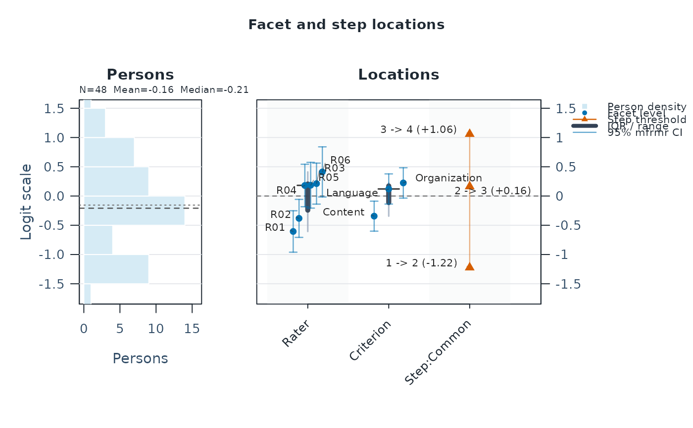# Save the summary, then display its tables
results <- summary(fit)
results$person_overview # One row summarizing person ability estimates
#> # A tibble: 1 × 11
#>   Persons DistributionN ReviewExcludedExtremeE…¹ EstimateUse   Mean    SD Median
#>     <int>         <int>                    <int> <chr>        <dbl> <dbl>  <dbl>
#> 1      48            48                        0 source_fit… -0.155 0.824 -0.208
#> # ℹ abbreviated name: ¹​ReviewExcludedExtremeEAPs
#> # ℹ 4 more variables: Min <dbl>, Max <dbl>, Span <dbl>, MeanPosteriorSD <dbl>
results$facet_overview  # One row per facet: number of levels, mean, SD, range
#> # A tibble: 2 × 7
#>   Facet     Levels MeanEstimate SDEstimate MinEstimate MaxEstimate  Span
#>   <chr>      <int>        <dbl>      <dbl>       <dbl>       <dbl> <dbl>
#> 1 Criterion      3            0      0.302      -0.344       0.224 0.568
#> 2 Rater          6            0      0.399      -0.606       0.412 1.02 

# Check the interpretation status and recommended next step
results$decision
#>                                                           Interpretation
#> 1 Fit-readiness requirements satisfied; formal precision review required
#>   FormalInference FitReadiness                                              Why
#> 1              No        ready Formal precision support has not been evaluated.
#>                                                                                                                                                   NextAction
#> 1 Run `diagnose_mfrm()` and pass its result as `diagnostics =` to evaluate formal precision support; fit readiness alone is not a formal-inference decision.
# }