
This vignette covers the package-native route for:
- checking whether a design is connected enough for a common scale
- exporting anchor candidates from an existing fit
- screening differential facet functioning (DFF)
- deciding whether subgroup contrasts are linked and available for screening
For a broader workflow guide, see
vignette("mfrmr-workflow", package = "mfrmr"). For the
shorter help-page map, see
help("mfrmr_linking_and_dff", package = "mfrmr").
Start with the assignment, before fitting
There are two different meanings of an anchor. A common
person supplies ratings that connect raters; their ability can
remain unknown and estimated. A fixed anchor supplies a
known parameter value to fit_mfrm(anchors = ...). The
latter is not needed merely because several raters score the same
person.
For example, the following existing simulation routes describe three practical assignments. Four common persons and eight raters illustrate the syntax; they are not recommended minimum counts. The common-person example uses more rating rows than the other examples, so this is not an equal-budget precision comparison.
library(mfrmr)

common <- build_mfrm_sim_spec(
  n_person = 40, n_rater = 8, n_criterion = 3, raters_per_person = 2,
  assignment = "sparse_linked",
  sparse_controls = list(link_persons = 4, link_raters_per_person = 8,
                         assignment_mode = "balanced")
)
rotating <- build_mfrm_sim_spec(
  n_person = 40, n_rater = 8, n_criterion = 3, raters_per_person = 2,
  assignment = "rotating"
)
random <- build_mfrm_sim_spec(
  n_person = 40, n_rater = 8, n_criterion = 3, raters_per_person = 2,
  assignment = "sparse_linked",
  sparse_controls = list(link_persons = 0, assignment_mode = "random")
)

# Use common, rotating, or random here to inspect the chosen assignment.
ratings <- simulate_mfrm_data(sim_spec = common, seed = 27309)
data_review <- describe_mfrm_data(
  ratings, person = "Person", facets = c("Rater", "Criterion"),
  score = "Score", include_agreement = FALSE
)
data_review$design_connectivity
#>      Basis     Facet PersonNodes FacetLevelNodes Edges Components
#> 1 observed     Rater          40               8   104          1
#> 2 observed Criterion          40               3   120          1
#>   LargestComponentPersons LargestComponentLevels LargestComponentPercent
#> 1                      40                      8                     100
#> 2                      40                      3                     100
#>   Connected
#> 1      TRUE
#> 2      TRUE
The common-person design gives four persons all eight raters and the
other 36 persons two raters each. The rotating and random designs give
each person two raters. A random draw does not guarantee that all raters
are connected or equally busy. For actual data, supply the planned
assignment to describe_mfrm_data(expected_design = ...) to
distinguish missing assigned ratings from cells that were never
assigned.
Eckes’s discussion of rating designs distinguishes distributed
overlap, a single common examinee, disconnected groups and task-nested
spiral assignments (2023 edition, Section 9.1, Table 9.1, pp. 151–155).
The rotating generator here uses the selected raters on all generated
criteria. Use an explicit design_skeleton for task-specific
assignments; do not equate ordinary rotation with every spiral design.
Check model identification as well as graph connections, especially when
raters are nested within tasks.
Connectedness means paths exist, not that those paths carry enough information. Review reliance on a small linking set, its composition, and sensitivity to loss of a linking person or rater. The ability to generate a sparse design is not a guarantee that a particular estimator or its intervals work well for it.
Fit and diagnose the observed ratings
library(mfrmr)

bias_df <- load_mfrmr_data("example_bias")

# This example uses compact quadrature for a shorter runtime.
# For final DFF or linking evidence, refit with the package default or a higher
# quadrature setting and record that setting in the analysis log.
fit <- fit_mfrm(
  bias_df,
  person = "Person",
  facets = c("Rater", "Criterion"),
  score = "Score",
  method = "MML",
  model = "RSM",
  quad_points = 31
)

diag <- diagnose_mfrm(fit, residual_pca = "none")
1. Check connectedness first
Use subset_connectivity_report() before interpreting
subgroup or cross-form contrasts.
sc <- subset_connectivity_report(fit, diagnostics = diag)

sc$summary[, c("Subset", "Observations", "ObservationPercent")]
#>   Subset Observations ObservationPercent
#> 1      1          384                100
plot(sc, type = "design_matrix", preset = "publication")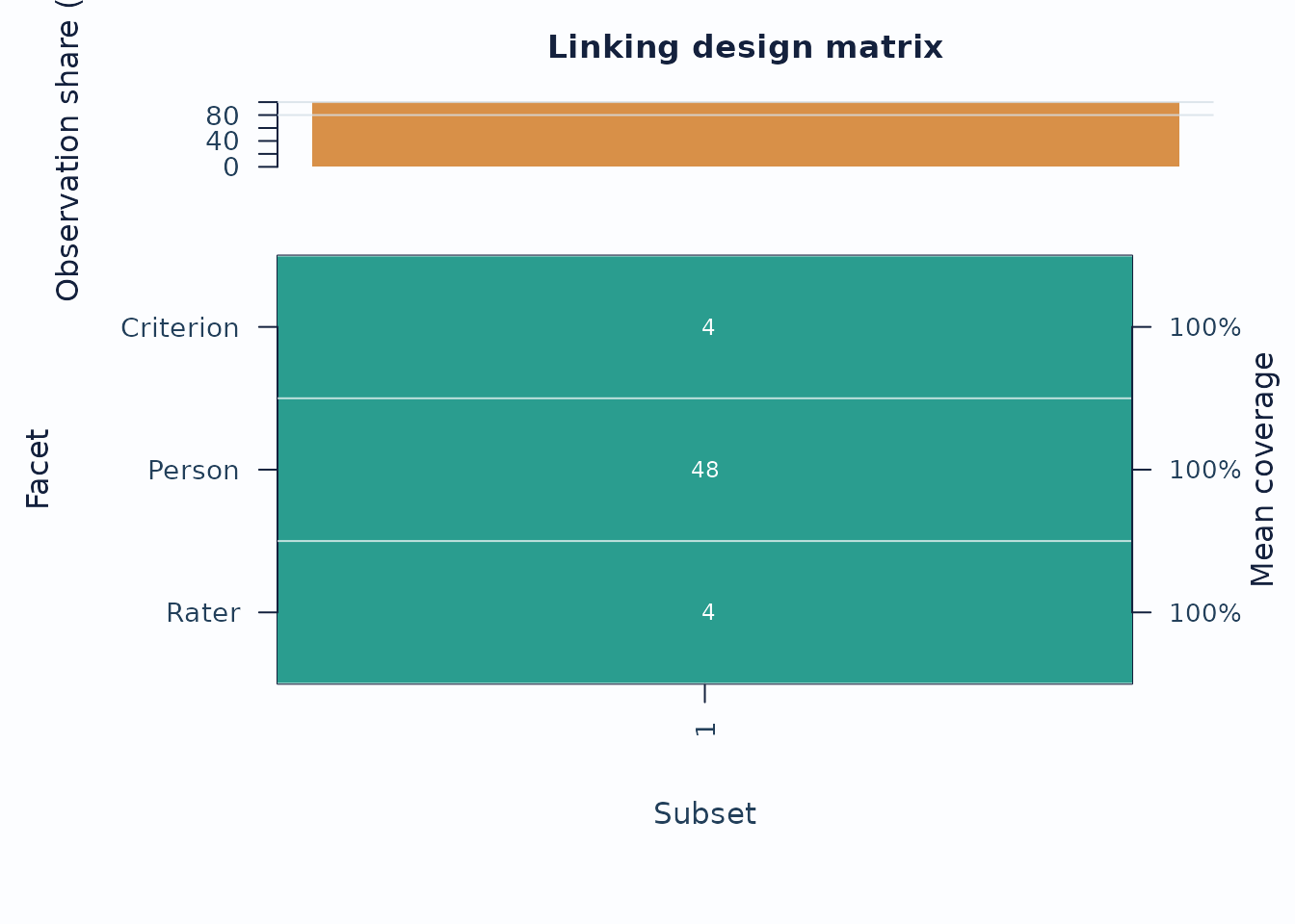
Interpretation:
- Sparse rows or columns indicate weaker design coverage.
- Weak coverage should lower confidence in subgroup comparisons.
- Use the co-observation design graph, not rater agreement, severity-direction, or halo response networks, to assess empirical connectedness. Response-network correlations do not create a common scale.
2. Export anchor candidates
make_anchor_table() mechanically exports fitted values
in the direct-anchor schema. Its output is a candidate table, not a
validated anchor set.
anchors <- make_anchor_table(fit, facets = "Criterion")
head(anchors)
#> # A tibble: 4 × 3
#>   Facet     Level         Anchor
#>   <chr>     <chr>          <dbl>
#> 1 Criterion Accuracy      0.524
#> 2 Criterion Content      -0.199
#> 3 Criterion Language     -0.275
#> 4 Criterion Organization -0.0499
By default, make_anchor_table() refuses a source whose
current readiness record does not have
InferenceReady = TRUE. Use
readiness_policy = "review" only to inspect review-only
candidate values, not to reuse them as anchors. For a ready reference
fit, also document cross-run element identity and invariance and confirm
compatible model, score, orientation, and population conventions. Then
use review_mfrm_anchors() to check table syntax and
receiving-data support. That review does not certify the substantive
link.
Keep the roles distinct: common ratings or common elements supply
observed design overlap; anchors fix individual parameters;
group_anchors constrain a group mean under an externally
justified target or equal-mean assumption. Neither constraint type
manufactures empirical overlap.
Design the link, not only the percentage
No anchor percentage or count is universally adequate. In sparse designs, link quality also depends on coverage, the distribution and redundancy of the links, whether one articulation point or critical edge holds the network together, the location and model fit of the linking set, and the intended use of ranks or classifications. Inspect both Rater-centered and Person/task- centered assignment graphs rather than treating a minimum count as proof of a common scale. This distinction is consistent with work on sparse linking networks by Myford and Wolfe (2000), Wind and Jones (2018), and Uto (2021).
Fixed anchor values also carry uncertainty from their source calibration. Current mfrmr drift and chain summaries do not propagate every source-fit, offset, and cross-fit covariance component. When results depend on the anchor set, compare defensible alternatives and report that sensitivity; fixed- parameter calibration error should not be mistaken for zero uncertainty (Robitzsch, 2024).
3. Compare group residuals
Residual comparisons describe how observed-minus-expected scores differ between groups. They use score units and do not test differential functioning.
A group with higher average ability can score higher without differential functioning. DFF concerns a facet difference at the same ability. Residual screens inherit the fitted population assumptions, and fixed-standard-normal RSM/PCM subgroup refits do not estimate group ability distributions. Linking anchors alone do not address an omitted group difference. Review these assumptions before interpreting a residual difference involving a rater or criterion.
Representing group ability differences is necessary for a suitable population model, but does not turn the current residual screen into a calibrated DFF test. MML residuals evaluate expected scores at EAP ability estimates. Because the response function is nonlinear, a no-DFF model can still have different mean residuals across groups. This concerns the null being tested as well as its standard error.
The residual method therefore returns no p-values, confidence
intervals or positive/negative classifications. For compatibility, its
former SE and test columns contain NA. Recompute older
residual results with analyze_dff() using the existing fit
and original data; no model refit is needed.
dff_resid <- analyze_dff(
  fit,
  diag,
  facet = "Criterion",
  group = "Group",
  data = bias_df,
  method = "residual"
)

dff_resid$summary
#> # A tibble: 2 × 2
#>   Classification    Count
#>   <chr>             <int>
#> 1 Residual contrast     4
#> 2 Unavailable           0
head(
  dff_resid$dif_table[, c("Level", "Group1", "Group2", "Contrast", "N_Group1", "N_Group2")],
  8
)
#> # A tibble: 4 × 6
#>   Level        Group1 Group2 Contrast N_Group1 N_Group2
#>   <chr>        <chr>  <chr>     <dbl>    <int>    <int>
#> 1 Accuracy     A      B        0.403        48       48
#> 2 Content      A      B       -0.0643       48       48
#> 3 Language     A      B       -0.401        48       48
#> 4 Organization A      B       -0.101        48       48
plot_dif_heatmap(dff_resid)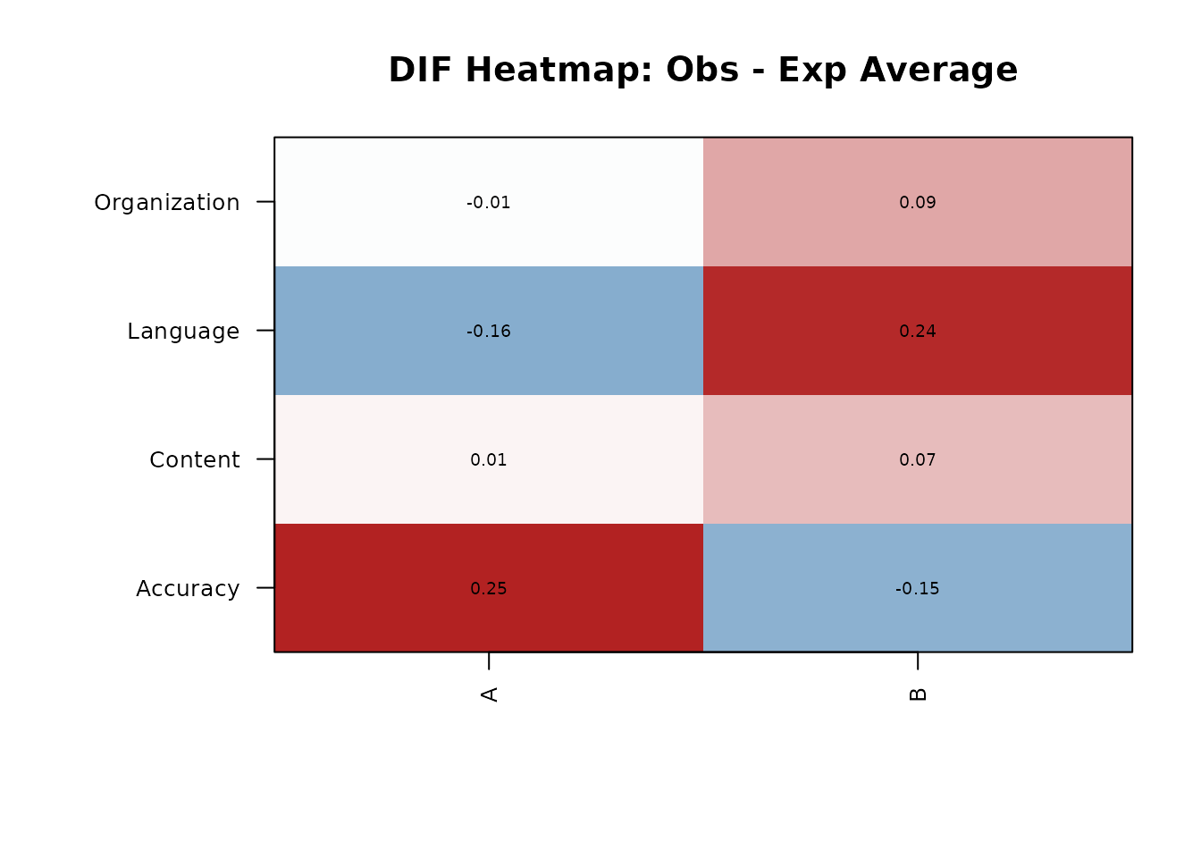
Interpretation:
- Read
Contrastas the residual mean in Group1 minus that in Group2. - A positive value means higher residual scores in Group1, not greater rater leniency.
- Reserve
ScaleLinkStatusandContrastComparablefor refit-based contrasts.
4. Refit DFF when subgroup comparisons are defensible
The refit route reports logit-scale point contrasts when subgroup
linking supports a common scale. Any available SE or test statistic
conditions on the baseline anchors and omits their uncertainty and
cross-refit covariance; FormalInferenceEligible remains
FALSE, even with adequate linking. The default refit
linking screen requires at least five anchored levels in total across
the non-target linking facets in each subgroup. A weak link withholds
contrast SEs and p-values. Inspect LinkingAnchoredLevels,
LinkingThreshold, and ScaleLinkStatus; five is
a local screening threshold, not a universal adequate anchor count or
proof of invariance.
Refits currently refuse baselines with user-specified active
population models, fitted facet interactions, or group-anchor
constraints because those structures cannot yet be replayed and linked
completely within subgroups. The default GPCM-MML identification
intercept is handled separately. Residual DFF remains a screening
alternative; see ?analyze_dff for the exact scope.
dff_refit <- analyze_dff(
  fit,
  diag,
  facet = "Criterion",
  group = "Group",
  data = bias_df,
  method = "refit"
)

dff_refit$summary
#> # A tibble: 2 × 2
#>   Classification                      Count
#>   <chr>                               <int>
#> 1 Linked contrast (screening only)        0
#> 2 Unclassified (insufficient linking)     4
head(
  dff_refit$dif_table[, c("Level", "Group1", "Group2", "Classification", "ContrastComparable")],
  8
)
#> # A tibble: 4 × 5
#>   Level        Group1 Group2 Classification                   ContrastComparable
#>   <chr>        <chr>  <chr>  <chr>                            <lgl>
#> 1 Accuracy     A      B      Unclassified (insufficient link… FALSE
#> 2 Content      A      B      Unclassified (insufficient link… FALSE
#> 3 Language     A      B      Unclassified (insufficient link… FALSE
#> 4 Organization A      B      Unclassified (insufficient link… FALSE
5. Cell-level follow-up
If the level-wise screen points to a specific facet, follow up with the interaction table and narrative report.
dit <- dif_interaction_table(
  fit,
  diag,
  facet = "Criterion",
  group = "Group",
  data = bias_df
)

head(dit$table)
#> # A tibble: 6 × 18
#>   Level  GroupValue     N ObsScore ExpScore ObsExpAvg Var_sum sparse StdResidual
#>   <chr>  <chr>      <int>    <int>    <dbl>     <dbl>   <dbl> <lgl>        <dbl>
#> 1 Accur… A             48      125     113.    0.255     28.6 FALSE        2.29
#> 2 Accur… B             48      117     124.   -0.147     29.2 FALSE       -1.31
#> 3 Conte… A             48      134     133.    0.0131    27.8 FALSE        0.119
#> 4 Conte… B             48      148     144.    0.0774    26.1 FALSE        0.727
#> 5 Langu… A             48      128     135.   -0.156     27.5 FALSE       -1.43
#> 6 Langu… B             48      158     146.    0.245     25.6 FALSE        2.32
#> # ℹ 9 more variables: t <dbl>, df <dbl>, p_value <dbl>,
#> #   FormalInferenceEligible <lgl>, ReportingUse <chr>, Interpretation <chr>,
#> #   p_adjusted <dbl>, flag_t <lgl>, flag_bias <lgl>

dr <- dif_report(dff_resid)
cat(dr$narrative)
#> Mean observed-minus-expected scores were compared for the Criterion facet across levels of Group. 4 of 4 group comparisons had sufficient observations to report a residual difference. Differences are in score units. They do not isolate differential functioning: group residual means can differ even when response parameters are the same. No p-values, confidence intervals or positive/negative classifications are provided.
6. Model-estimated facet interactions
Residual bias and DFF tools screen for unusual cells after fitting
the additive model. When the interaction hypothesis is specified in
advance, use facet_interactions to estimate the named
two-way non-person facet interaction in the model likelihood.
fit_add <- fit_mfrm(
  bias_df,
  person = "Person",
  facets = c("Rater", "Criterion"),
  score = "Score",
  method = "MML",
  model = "RSM",
  quad_points = 7
)

fit_interaction <- fit_mfrm(
  bias_df,
  person = "Person",
  facets = c("Rater", "Criterion"),
  score = "Score",
  method = "MML",
  model = "RSM",
  facet_interactions = "Rater:Criterion",
  quad_points = 31
)

interaction_effect_table(fit_interaction)
compare_mfrm(Additive = fit_add, Interaction = fit_interaction, nested = TRUE)
Interpretation:
- Name the facet pair explicitly before fitting.
- Treat the interaction estimates as fixed-effect deviations from the additive MFRM under zero marginal-sum constraints.
- Inspect sparse interaction cells before reporting substantive claims.
- Keep this route separate from residual screening with
estimate_bias().
7. Multi-wave anchor review
When you work across administrations, the route usually moves from a
declared common-anchor design to anchored fitting and then to drift
review. The block below is schematic: wave1 and
wave2 must be administrations for which the listed facet
levels have documented cross-wave identity and unchanged meaning.
Do not substitute ej2021_study1 and
ej2021_study2 here. They are independent legacy synthetic
studies; reused raw labels do not identify common persons, raters, or
anchors and do not link their scales.
declared_common_facets <- c("Criterion")

fit1 <- fit_mfrm(
  wave1, "Person", c("Rater", "Criterion"), "Score",
  method = "MML"
)

anchored <- anchor_to_baseline(
  wave2,
  fit1,
  person = "Person",
  facets = c("Rater", "Criterion"),
  score = "Score",
  anchor_facets = declared_common_facets
)

fit2 <- fit_mfrm(
  wave2, "Person", c("Rater", "Criterion"), "Score",
  method = "MML"
)
drift <- detect_anchor_drift(list(Wave1 = fit1, Wave2 = fit2))
plot_anchor_drift(drift, type = "drift", preset = "publication")
The current drift and chain helpers estimate one pooled offset across
every selected common element and facet. Their SE ratios do not include
uncertainty from estimating that offset or cross-fit covariance, and
cumulative chain offsets have no propagated SE. Offset_SD
is residual spread rather than an offset standard error. Use one
coherent linking facet unless a common shift across facet blocks is
defensible, and treat flags and support counts as review screens rather
than formal tests or proof of scale equivalence.
Recommended sequence
For a compact linking route:
fit_mfrm()diagnose_mfrm()subset_connectivity_report()-
make_anchor_table()orreview_mfrm_anchors() analyze_dff()-
dif_report()andplot_dif_heatmap() -
interaction_effect_table()after a confirmatoryfacet_interactionsfit -
anchor_to_baseline()/detect_anchor_drift()when working across waves
References
- Myford, C. M., & Wolfe, E. W. (2000). Strengthening the ties that bind: Improving the linking network in sparsely connected rating designs. ETS Research Report Series, 2000(1).
- Robitzsch, A. (2024). Bias and linking error in fixed item parameter calibration. AppliedMath, 4(3), 1181–1191.
- Uto, M. (2021). Accuracy of performance-test linking based on a many-facet Rasch model. Behavior Research Methods, 53(4), 1440–1454.
- Wind, S. A., & Jones, E. (2018). The stabilizing influences of linking set size and model–data fit in sparse rater-mediated assessment networks. Educational and Psychological Measurement, 78(4), 679–707.