
A useful report explains the question, why the scoring design and
model can answer it, what the results show, and how far the answer
applies. This guide connects those steps to actual mfrmr
tables and figures. The Manuscript
coverage map also identifies information that the researcher must
provide outside the fitted model.
The running question is: after accounting for person ability
and criterion difficulty, how much do the raters differ in
severity? The synthetic data illustrate the reporting workflow;
they are not evidence about a real assessment or population. For loading
your own CSV, see
vignette("mfrmr-workflow", package = "mfrmr").
1. Fit once and retain the analysis record
# Load the package and synthetic ratings
library(mfrmr)
toy <- load_mfrmr_data("example_operational")
head(toy)
#>                Study Person Rater    Criterion Score Group
#> 1 OperationalExample   P001   R01     Language     4     A
#> 2 OperationalExample   P001   R01 Organization     2     A
#> 3 OperationalExample   P001   R02      Content     4     A
#> 4 OperationalExample   P001   R02     Language     3     A
#> 5 OperationalExample   P001   R02 Organization     2     A
#> 6 OperationalExample   P002   R01      Content     3     A

# Estimate person ability, rater severity, and criterion difficulty
fit <- fit_mfrm(
  data = toy,
  person = "Person",
  facets = c("Rater", "Criterion"),
  score = "Score",
  method = "MML",
  model = "RSM"
)

# Reuse these diagnostics in the tables and report below
diag <- diagnose_mfrm(fit, diagnostic_mode = "both", residual_pca = "none")
results <- summary(fit, diagnostics = diag)
One row is one rating. The rubric uses 1 to 4, and
all four categories occur. The example has 48 persons, six raters, and
three criteria, with 282 observed ratings. Here N is the
number of rating rows, not the number of independent participants.
Repeated ratings from the same person share that person’s latent ability
in the model.
MML means marginal maximum likelihood; RSM is a rating-scale model with shared category thresholds. In this default fit, the person distribution is fixed to standard normal, person scores are expected a posteriori (EAP) estimates, and rater and criterion effects are fixed parameters centered within each facet. Higher rater estimates mean stricter ratings, in logits. In a real study, explain why this population assumption and shared-threshold rubric match the question. Record any different estimator, constraints, anchors, weights, interactions, or score orientation.
results$overview[, c("Model", "Method", "N", "Persons", "Converged")]
#> # A tibble: 1 × 5
#>   Model Method     N Persons Converged
#>   <chr> <chr>  <dbl>   <int> <lgl>
#> 1 RSM   MML      282      48 TRUE
results$settings_overview[, c(
  "QuadPoints", "RatingMin", "RatingMax", "RatingRangeSource", "NoncenterFacet"
)]
#> # A tibble: 1 × 5
#>   QuadPoints RatingMin RatingMax RatingRangeSource NoncenterFacet
#>        <int>     <dbl>     <dbl> <chr>             <chr>
#> 1         31         1         4 observed          Person
results$row_retention
#>                             Stage Rows DroppedRows
#> 1          input_selected_columns  282           0
#> 2 after_missing_and_weight_filter  282           0
#>                            DroppedReason
#> 1
#> 2 missing values or non-positive weights
results$decision
#>               Interpretation FormalInference FitReadiness
#> 1 Ready for formal inference             Yes        ready
#>                                           Why
#> 1 All stored fit-readiness components passed.
#>                                                                                                                                                                   NextAction
#> 1 After reviewing convergence, run `review <- summary(fit, profile = "facets", detail = "brief")` for the comprehensive measurement review; FACETS software is not required.

# Record the iteration limit, integration grid, and numerical stopping details
spec <- specifications_report(fit)
spec$convergence_control
#>               Setting                                           Value
#> 1       MaxIterations                                             400
#> 2   RelativeTolerance                                           1e-09
#> 3          QuadPoints                                              31
#> 4   OptimizerCodeZero                                            TRUE
#> 5      InferenceReady                                            TRUE
#> 6 ConvergenceSeverity                                            pass
#> 7 FunctionEvaluations                                               7
#> 8    OptimizerMessage CONVERGENCE: REL_REDUCTION_OF_F <= FACTR*EPSMCH
results$overview[, c("OptimizerMethod", "ConvergenceStatus", "RequestedReltol", "EffectiveReltol")]
#> # A tibble: 1 × 4
#>   OptimizerMethod ConvergenceStatus RequestedReltol EffectiveReltol
#>   <chr>           <chr>                       <dbl>           <dbl>
#> 1 L-BFGS-B        converged             0.000000001           1e-13
The default numerical integration uses 31 quadrature points. Retain
the analysis script and recorded controls with the results; convergence
alone does not establish numerical stability or model adequacy. If the
conclusions hinge on a close model comparison, use
mml_quadrature_sensitivity() with a prespecified denser
common grid and report whether the conclusion changes.
Show what was planned, observed, and excluded
data("mfrmr_example_operational_design", package = "mfrmr")
data_review <- describe_mfrm_data(
  data = toy,
  person = "Person",
  facets = c("Rater", "Criterion"),
  score = "Score",
  rating_min = 1,
  rating_max = 4,
  keep_original = TRUE,
  expected_design = mfrmr_example_operational_design
)
data_summary <- summary(data_review)
data_summary$missing
#>      Column Missing
#> 1 Criterion       0
#> 2    Person       0
#> 3     Rater       0
#> 4     Score       0
data_summary$structural_missingness
#>     Status ExpectedCells ObservedCells MatchedCells MissingExpectedCells
#> 1 declared           288           282          282                    6
#>   UnexpectedObservedCells CoverageRate ExpectedOnlyPersons UnexpectedPersons
#> 1                       0    0.9791667                   0                 0
data_summary$design_connectivity
#>               Basis     Facet PersonNodes FacetLevelNodes Edges Components
#> 1          observed     Rater          48               6    96          1
#> 2          observed Criterion          48               3   144          1
#> 3 declared_expected     Rater          48               6    96          1
#> 4 declared_expected Criterion          48               3   144          1
#>   LargestComponentPersons LargestComponentLevels LargestComponentPercent
#> 1                      48                      6                     100
#> 2                      48                      3                     100
#> 3                      48                      6                     100
#> 4                      48                      3                     100
#>   Connected
#> 1      TRUE
#> 2      TRUE
#> 3      TRUE
#> 4      TRUE

# Describe the scores and the amount of rating evidence
data_summary$score_distribution
#>   Score RawN WeightedN  Percent
#> 1     1   62        62 21.98582
#> 2     2   96        96 34.04255
#> 3     3   78        78 27.65957
#> 4     4   46        46 16.31206
data_summary$facet_overview
#>       Facet Levels TotalWeightedN MeanWeightedN MinWeightedN MaxWeightedN
#> 1 Criterion      3            282            94           94           94
#> 2     Rater      6            282            47           38           56
data.frame(MeanScore = mean(toy$Score), SDScore = sd(toy$Score))
#>   MeanScore  SDScore
#> 1  2.382979 1.002911
table(table(toy$Person)) # Number of persons with each observed rating count
#>
#>  5  6
#>  6 42
as.data.frame(results$person_overview[, c(
  "Persons", "DistributionN", "ReviewExcludedExtremeEAPs", "Mean", "SD", "MeanPosteriorSD"
)])
#>   Persons DistributionN ReviewExcludedExtremeEAPs       Mean        SD
#> 1      48            48                         0 -0.1554342 0.8236778
#>   MeanPosteriorSD
#> 1         0.47615
The supplied roster contains 288 planned rating cells, of which six
are absent. All 282 input rows are retained in fitting. These are
different counts: absent planned ratings are not rows discarded by
fit_mfrm(). Report the assignment scheme, overlap,
exclusions, and reasons for missing ratings. Without a roster, do not
label every unobserved person-by-rater combination as a missing planned
rating. A connected design is relevant to comparability, but does not
establish anchor invariance or sufficient precision.
These counts describe different units. In the example, 42 persons have six ratings and six have five; rater workloads range from 38 to 56 rating rows. For repeated testing, state whether a person ID identifies a person, a response, or an occasion, and how dependence across occasions is handled. Preserve the original rubric, any scoring exceptions, and the exact recoding rule. Such details affect what the model can answer: Goodwin (2016, Sections 3–4 and Table 1) documents score-use contexts, rating history, exclusions, and category recoding before reporting rater differences.
State which persons enter distribution summaries. Eckes (2005, Tables
1–2) marks summaries restricted to nonextreme examinees. In this example
the person summary includes all 48 persons. SD describes
variation across person EAP estimates; MeanPosteriorSD
describes their average within-person uncertainty. They are not
interchangeable, and neither is a rater or criterion SE.
2. Check uncertainty and fit before writing the answer
prec <- precision_review_report(fit, diagnostics = diag)
prec$profile[, c(
  "PrecisionTier", "SupportsFormalInference", "PersonSEBasis", "NonPersonSEBasis"
)]
#>   PrecisionTier SupportsFormalInference      PersonSEBasis
#> 1   model_based                    TRUE Posterior SD (EAP)
#>             NonPersonSEBasis
#> 1 Observed information (MML)
prec$checks
#>                      Check Status
#> 1           Precision tier   pass
#> 2    Optimizer convergence   pass
#> 3     ModelSE availability   pass
#> 4 Fit-adjusted SE ordering   pass
#> 5     Reliability ordering   pass
#> 6 Facet precision coverage   pass
#> 7         SE source labels   pass
#>                                                                                                                                                                                                    Detail
#> 1 Uncertainty is conditional on the fitted model. Person posterior SDs condition on the fitted calibration; facet standard errors use observed information. Review interval assumptions before reporting.
#> 2                                                                                                              Numerical convergence checks passed; this alone does not establish valid SEs or intervals.
#> 3                                                                                                                                     Finite standard errors were available for 100.0% of non-fixed rows.
#> 4                                                                                                              Among available pairs, fit-adjusted SEs were at least as large as their unadjusted values.
#> 5                                                                                                     Among available pairs, fit-adjusted reliability values were not larger than the model-based values.
#> 6                                                                                                                    Each facet had sample/population summaries for both model and fit-adjusted SE modes.
#> 7                                                                                                                     Person uncertainty uses posterior SDs; facet uncertainty uses observed information.

# These diagnostics address departures from the fitted response model
diag_summary <- summary(diag)
diag_summary$overall_fit
#> # A tibble: 1 × 6
#>   Infit Outfit InfitZSTD OutfitZSTD DF_Infit DF_Outfit
#>   <dbl>  <dbl>     <dbl>      <dbl>    <dbl>     <dbl>
#> 1 0.866  0.857     -1.28      -1.75     174.       282
diag_summary$diagnostic_basis[, c("DiagnosticPath", "Status", "ReportingUse")]
#> # A tibble: 4 × 3
#>   DiagnosticPath                   Status        ReportingUse
#>   <chr>                            <chr>         <chr>
#> 1 legacy_residual_fit              computed      legacy_compatibility_screen
#> 2 strict_marginal_fit              computed      screening_only
#> 3 strict_pairwise_local_dependence computed      screening_only
#> 4 posterior_predictive_follow_up   not_available screening_only
Read results$decision, including Why and
NextAction, together with these checks. A
model_based precision tier describes the uncertainty
calculation; it does not by itself justify every inferential claim.
Retain restrictions reported for the fit, design, or particular
statistic. For this fit, person uncertainty is posterior SD and
non-person SEs use observed information.
Infit and Outfit have a reference value of 1 and summarize departures
from the model. Report the statistics and the source and purpose of any
review cutoff; a flag is not an automatic exclusion rule. Global fit can
hide local problems. The default diagnostic_mode = "both"
retains residual/EAP diagnostics and latent-integrated marginal screens.
Their reference bases differ; inspect
prec$fit_separation_basis before describing MnSq, ZSTD,
separation, or reliability as if they were a single adequacy test.
When reporting the frequency of large residuals, state the rule and denominator. For example, Eckes (2005, p. 204) reports counts at two absolute standardized- residual cutoffs. The following shows those descriptive counts for the current EAP-residual path:
z <- diag$obs$StdResidual
residual_counts <- data.frame(
  AbsoluteZCutoff = c(2, 3),
  Evaluated = sum(is.finite(z)),
  Unavailable = sum(!is.finite(z)),
  Flagged = c(sum(abs(z[is.finite(z)]) >= 2),
              sum(abs(z[is.finite(z)]) >= 3))
)
residual_counts$Percent <- 100 * residual_counts$Flagged / residual_counts$Evaluated
residual_counts
#>   AbsoluteZCutoff Evaluated Unavailable Flagged   Percent
#> 1               2       282           0       7 2.4822695
#> 2               3       282           0       1 0.3546099
Use the residual basis appropriate to your analysis. These are
descriptive tail counts, not a calibrated global test or a universal
rule that a certain percentage establishes fit. The observed-category
probability screen in unexpected_response_table() is an
additional rule unless explicitly disabled; its default count is not the
same as counting only abs(StdResidual) >= 2.
Keep the marginal screening results visible alongside those counts:
diag_summary$marginal_fit[, c(
  "OverallRMSD", "StepGroupsFlagged", "FacetLevelsFlagged",
  "PairwiseFlaggedLevelPairs", "ReportingUse"
)]
#> # A tibble: 1 × 5
#>   OverallRMSD StepGroupsFlagged FacetLevelsFlagged PairwiseFlaggedLevelPairs
#>         <dbl>             <int>              <int>                     <int>
#> 1     0.00624                 0                  1                         1
#> # ℹ 1 more variable: ReportingUse <chr>
diag$marginal_fit$thresholds
#> $abs_z_warn
#> [1] 2
#>
#> $rmsd_warn
#> [1] 0.05
diag$marginal_fit$pairwise$thresholds
#> $abs_z_warn
#> [1] 2
#>
#> $exact_gap_warn
#> [1] 0.1
#>
#> $adjacent_gap_warn
#> [1] 0.1
subset(diag$marginal_fit$facet_level$summary_stats, Flagged,
       c("Facet", "Level", "GroupCount", "RMSD", "MaxAbsStdResidual"))
#> # A tibble: 1 × 5
#>   Facet Level GroupCount   RMSD MaxAbsStdResidual
#>   <chr> <chr>      <dbl>  <dbl>             <dbl>
#> 1 Rater R06           38 0.0512              1.09
subset(diag$marginal_fit$pairwise$pair_stats, Flagged,
       c("Facet", "Level1", "Level2", "LevelPairCount", "ExactAgreement", "ExpectedExactAgreement"))
#> # A tibble: 1 × 6
#>   Facet Level1 Level2 LevelPairCount ExactAgreement ExpectedExactAgreement
#>   <chr> <chr>  <chr>           <int>          <dbl>                  <dbl>
#> 1 Rater R04    R05                23          0.609                  0.398
The package’s default marginal rules use an absolute
standardized-residual cutoff of 2 or a root-mean-square proportion
discrepancy of 0.05; pairwise screens also use an exact/adjacent
agreement-gap cutoff of 0.10. Record the rules used in your run and
inspect flagged groups with plot_marginal_fit() and
plot_marginal_pairwise(). These remain screening results;
an acceptable overall average does not resolve local warnings.
3. Show estimates, uncertainty, and the answer
measurements <- fit_measures_table(fit, diagnostics = diag, ci_level = 0.95)
rater_table <- subset(
  measurements$table, Facet == "Rater",
  c("Level", "N", "Measure", "SE", "CI_Lower", "CI_Upper", "Infit", "Outfit")
)
rater_table <- rater_table[order(rater_table$Measure), ]

rater_apa <- apa_table(
  rater_table,
  digits = 3,
  caption = "Rater severity and fit in the synthetic MML/RSM example",
  note = paste(
    "282 ratings of 48 persons by six raters on three criteria using a 1-4 rubric.",
    "N counts rating rows. Measures and SEs are in logits; higher values mean stricter ratings.",
    "Intervals are 95% normal approximations from observed-information SEs.",
    "Rater effects are centered within facet. Infit and Outfit have reference value 1."
  )
)
rater_apa
#> Rater severity and fit in the synthetic MML/RSM example
#>  Level  N Measure    SE CI_Lower CI_Upper Infit Outfit
#>    R01 47  -0.606 0.224   -1.046   -0.166 0.772  0.757
#>    R02 56  -0.382 0.209   -0.791    0.027 0.954  1.015
#>    R04 47   0.180 0.223   -0.256    0.616 0.917  0.891
#>    R05 44   0.184 0.234   -0.275    0.643 0.648  0.640
#>    R03 50   0.212 0.217   -0.212    0.637 1.011  0.981
#>    R06 38   0.412 0.249   -0.077    0.901 0.820  0.798
#> Note. 282 ratings of 48 persons by six raters on three criteria using a 1-4 rubric. N counts rating rows. Measures and SEs are in logits; higher values mean stricter ratings. Intervals are 95% normal approximations from observed-information SEs. Rater effects are centered within facet. Infit and Outfit have reference value 1.

# Display the estimates on the common logit scale
plot(fit, diagnostics = diag, show_ci = TRUE)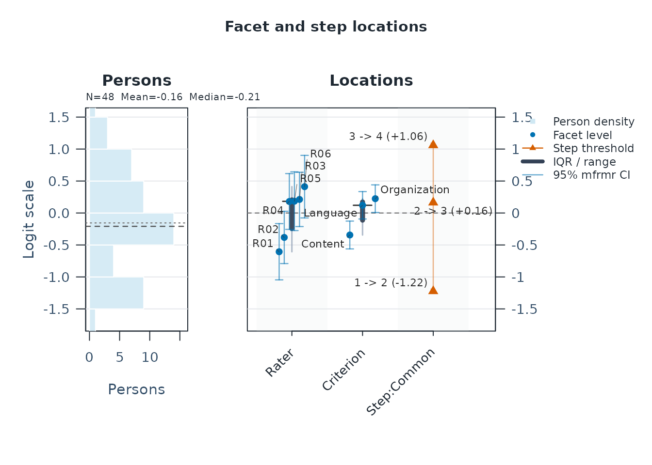
Pass the same diag to the table and plot so their
intervals use the same SEs. Without diagnostics, Wright-map
intervals use exploratory observation-table SEs, which can differ from
the MML observed-information SEs reported here. Steps on this map are
point estimates; their uncertainty is reported in the separate threshold
table below.
apa_table() prints the table, caption, and note; its
$table member holds the data for further formatting.
digits rounds all numeric columns uniformly. Review
statistic-specific rounding, especially for p values and
intervals, and the target journal’s format before submission.
A worked explanation for this synthetic example is:
We asked how much raters differed in severity after accounting for person ability and criterion difficulty. The model includes those facets so that raw rater averages are not the only basis for comparison. Estimated rater severity ranged from -0.606 logits (R01; SE = 0.224, 95% CI [-1.046, -0.166]) to 0.412 logits (R06; SE = 0.249, 95% CI [-0.077, 0.901]), a span of about 1.018 logits. Thus, the fitted model describes R06 as stricter than R01 in these data. This span is descriptive: it is not an interval or a hypothesis test for the difference. The evidence does not establish why the raters differ or how much a particular examinee’s decision would change.
The intervals compare each centered rater effect with its reference; their overlap is not a pairwise test. A contrast needs uncertainty for that contrast, including covariance, and a multiplicity plan if several comparisons are made. Whether a difference matters in practice depends on the rubric, the score use, and any decision rule. Do not convert a logit span directly into rubric points or claim that severity differences prove biased or inconsistent scoring. For person tables, state the EAP/posterior-SD basis and the interval method explicitly; normal approximations are not posterior quantile intervals.
Keep separation, agreement, and category functioning distinct
apa_table(
  diag_summary$reliability[, c("Facet", "Levels", "Separation", "Strata", "Reliability", "RealReliability")],
  digits = 3,
  caption = "Separation and reliability by facet",
  note = "Interpret the facet and error basis explicitly; rater separation reliability is not interrater agreement."
)
#> Warning: Unknown or uninitialised column: `config`.
#> Separation and reliability by facet
#>      Facet Levels Separation Strata Reliability RealReliability
#>  Criterion      3      2.555  3.740       0.867           0.866
#>     Person     48      1.406  2.207       0.664           0.614
#>      Rater      6      1.449  2.265       0.677           0.677
#> Note. Interpret the facet and error basis explicitly; rater separation reliability is not interrater agreement.

agreement <- interrater_agreement_table(fit, diagnostics = diag)
agreement$summary[, c(
  "OpportunityCount", "ExactAgreement", "ExpectedExactAgreement", "AdjacentAgreement"
)]
#>   OpportunityCount ExactAgreement ExpectedExactAgreement AdjacentAgreement
#> 1              138      0.3913043              0.3507673         0.8550725
A rater separation reliability describes how distinctly rater
locations are estimated relative to their errors; a high value does not
mean that raters agree. Person separation reliability addresses
differentiation among persons under its stated error basis. Specify
whether the model or misfit-adjusted (RealReliability)
index is reported, and the replication/error sources relevant to the
intended score use. These coefficients do not describe every possible
source of measurement error.
Also identify the formula. In diag$reliability,
Reliability is the separation-based ratio
max(V - E, 0) / V, where V is the sample
variance of finite facet estimates and E is the mean
squared model SE over available SEs. The ratio is unavailable when
V is zero or unavailable. Separation is
sqrt(max(V - E, 0) / E) when defined, and
Strata is (4 * Separation + 1) / 3; they are
distinct indices, not observed groups. The underlying quantities are
available directly:
diag$reliability[, c("Facet", "Levels", "ObservedVariance", "ModelErrorVariance", "Reliability")]
#> # A tibble: 3 × 5
#>   Facet     Levels ObservedVariance ModelErrorVariance Reliability
#>   <chr>      <int>            <dbl>              <dbl>       <dbl>
#> 1 Criterion      3           0.0915             0.0122       0.867
#> 2 Person        48           0.678              0.228        0.664
#> 3 Rater          6           0.159              0.0512       0.677
This is not the posterior-variance EAP reliability reported by Xiao et al. (2026, Section 2.5, Equation 4), whose denominator combines the spread of EAP scores with posterior variances. Nor is it the squared correlation with known true abilities used in their simulation. Report the package’s coefficient under its own name and basis; numerical comparisons across papers require matching definitions and scoring designs. For example, this analysis’s person separation reliability is 0.664, not a TAM EAP-reliability estimate.
Here the observed exact agreement is 54/138 = 39.1% across available
paired ratings of the same person and criterion; adjacent agreement
(within one category) is 85.5%. ExpectedExactAgreement is
the fitted-model baseline (35.1% here), not an independent
chance-agreement correction. Report the opportunity count and overlap
pattern, not just a percentage. These are observed-score summaries; keep
them separate from the marginal diagnostic screens above. Use
agreement$pairs when differences among rater pairs
matter.
scale <- rating_scale_table(fit, diagnostics = diag)
scale$category_table[, c("Category", "Count", "AvgPersonMeasure", "Infit", "Outfit")]
#>   Category Count AvgPersonMeasure     Infit    Outfit
#> 1        1    62       -0.9209312 1.5434694 1.3053867
#> 2        2    96       -0.3314206 0.4933638 0.5214360
#> 3        3    78        0.1586824 0.3395566 0.3440066
#> 4        4    46        0.6843099 1.9416014 1.8255900
scale$threshold_table
#>     Step   Estimate StepFacet StepIndex   Spacing Ordered ThresholdMonotonic
#> 1 Step_1 -1.2229852    Common         1        NA      NA               TRUE
#> 2 Step_2  0.1634468    Common         2 1.3864320    TRUE               TRUE
#> 3 Step_3  1.0595384    Common         3 0.8960916    TRUE               TRUE
#>   GapFromPrev LowerCategory UpperCategory WeaklyIdentified ThresholdCaveat
#> 1          NA             1             2            FALSE
#> 2   1.3864320             2             3            FALSE
#> 3   0.8960916             3             4            FALSE
plot(scale)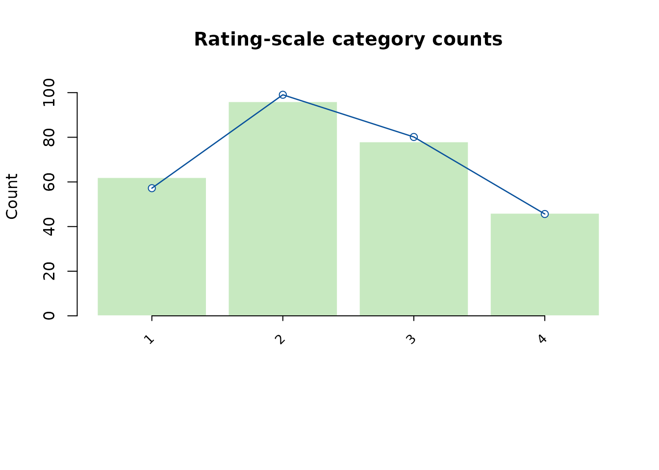
For a threshold table with uncertainty, use the diagnostics already computed:
steps <- diag$parameter_uncertainty$steps
steps[, c("Step", "Estimate", "SE", "CI_Lower", "CI_Upper", "CI_Level")]
#> # A tibble: 3 × 6
#>   Step   Estimate    SE CI_Lower CI_Upper CI_Level
#>   <chr>     <dbl> <dbl>    <dbl>    <dbl>    <dbl>
#> 1 Step_1   -1.22  0.169   -1.55    -0.892     0.95
#> 2 Step_2    0.163 0.167   -0.164    0.491     0.95
#> 3 Step_3    1.06  0.177    0.714    1.41      0.95
steps[, c("Step", "SE_Status", "CIEligible", "CIUse")]
#> # A tibble: 3 × 4
#>   Step   SE_Status CIEligible CIUse
#>   <chr>  <chr>     <lgl>      <chr>
#> 1 Step_1 ok        TRUE       primary_reporting
#> 2 Step_2 ok        TRUE       primary_reporting
#> 3 Step_3 ok TRUE primary_reportingStep_1, Step_2, and Step_3 are
the transitions 1–2, 2–3, and 3–4 here. The table uses MML
observed-information SEs and 95% normal intervals. A bare fit’s
steps table supplies point estimates;
rating_scale_table() does not automatically add the
uncertainty from a separately supplied diagnostics object. Check its
availability and reporting status before quoting intervals. For PCM,
retain StepFacet to identify the threshold family. Do not
substitute a criterion-location SE for a threshold SE, or a centered
step for the combined criterion-plus-step location. These distinctions
matter when preparing tables such as the criterion-specific thresholds
and SEs in Eckes (2005, Table 5).
The bars show observed category counts; the line shows fitted expected counts. Report category frequencies, threshold estimates and ordering, and any sparse or unused categories. Explain what the pattern means for the rubric. These checks can motivate rubric review; they do not automatically justify merging categories, changing scores, or claiming unidimensionality.
If the question concerns observed versus adjusted scores
Eckes (2005, Table 3) places observed scores, adjusted scores, logit measures, SEs, and rating counts together. State the adjustment reference when using a similar presentation. Here the reference is zero for the other facets:
fair <- fair_average_table(fit, diagnostics = diag, reference = "zero")
person_scores <- fair$raw_by_facet$Person
person_scores <- person_scores[order(person_scores$Level), ]
head(person_scores[, c(
  "Level", "TotalCount", "ObservedAverage", "FairZ", "Measure", "ModelSE"
)], 6)
#> # A tibble: 6 × 6
#>   Level TotalCount ObservedAverage FairZ Measure ModelSE
#>   <chr>      <int>           <dbl> <dbl>   <dbl>   <dbl>
#> 1 P001           5            3     2.68  0.284    0.486
#> 2 P002           6            3.33  2.95  0.661    0.484
#> 3 P003           6            2.83  2.49  0.0218   0.446
#> 4 P004           6            3     2.63  0.224    0.454
#> 5 P005           6            2.67  2.34 -0.175    0.442
#> 6 P006           5            3.4   2.96  0.677    0.526
These are the first six person IDs, selected for illustration.
FairZ is an expected score on the fitted 1–4 scale, at the
person’s estimated ability with the other facet references set to zero.
It is not a z-score. ModelSE here is the posterior SD of
person ability in logits, not the SE of FairZ. The RSM/PCM
fair_average_table() does not supply fair-score SEs. Its
mean-reference alternative, FairM, uses mean other-facet
measures; for non-person rows that also includes the mean person
measure. Neither averages over the actual assignment distribution.
A score-use claim needs the decision thresholds, rounding rule, reference environment, uncertainty treatment, and full-sample counts of changed decisions. The six-row preview is not that analysis. Statistical adjustment alone does not establish fairness or authorize replacing operational scores.
A short Methods and Results example
The following is an original write-up of this synthetic illustration, using the outputs above. It is not a reconstruction of any cited study. The research questions determine which of these supporting results belong in a real article’s main text or appendix.
Methods. We examined how much raters differed in severity after accounting for person ability and criterion difficulty. The synthetic dataset represented 48 persons, six raters, and three criteria scored from 1 to 4. Each person was assigned two raters across three criteria in an incomplete but connected design. Of 288 planned ratings, six were deliberately omitted in the example; all 282 observed ratings were retained. The raw rating mean was 2.38 (SD = 1.00), and individual raters contributed 38–56 ratings.
We fitted an RSM with person, rater, and criterion effects using
marginal maximum likelihood in mfrmr (software versions are
recorded below). Shared category steps represented a common transition
structure across criteria. The working person distribution was fixed to
standard normal, person scores were EAP estimates, and rater and
criterion effects were centered within facet. Higher rater estimates
indicated stricter scoring. The fit used 31 quadrature points, an
iteration limit of 400, and the recorded L-BFGS-B optimizer; the
requested relative tolerance was 1e-9 and the effective selected-stage
tolerance was 1e-13. We examined the stored readiness and precision
checks, residual/EAP and marginal diagnostics, and category use. Rater
and step intervals were 95% normal approximations from
observed-information SEs. Person uncertainty was reported as posterior
SD.
Results. The fit’s readiness and precision checks passed. Estimated rater severity spanned 1.018 logits, from -0.606 (R01; SE = 0.224) to 0.412 (R06; SE = 0.249); the individual intervals are reported in the rater table above. Thus, the fitted model described a range of rater severity after accounting for the included facets. This descriptive span did not test a pairwise contrast or quantify changes to assessment decisions.
Global residual-path Infit and Outfit were 0.866 and 0.857. Seven of 282 standardized residuals (2.48%) had absolute values of at least 2, and one (0.35%) reached 3. The marginal screens flagged R06 and the R04–R05 rater pair under the stated rules; these local signals require follow-up despite an overall marginal RMSD of 0.0062. Categories 1–4 occurred 62, 96, 78, and 46 times. Shared step estimates were ordered (-1.223, 0.163, and 1.060 logits; SEs = 0.169, 0.167, and 0.177). Person and rater separation reliabilities were 0.664 and 0.677. Observed exact agreement was 54/138 (39.1%) of available paired ratings of the same person and criterion; agreement within one category was 85.5%. These statistics describe distinct aspects of this fit. They do not establish the cause of severity differences, rubric validity, or the adequacy of an operational scoring decision. The illustration does not evaluate a different population model, a pairwise inferential contrast, or decision accuracy.
For an empirical report, add recruitment, participant and rater characteristics, training and scoring procedures, rubric rationale, actual missingness reasons, and the study-level information in the map below. Report unresolved diagnostics and relevant sensitivity results even if the optimizer converged. Never fill unknown study details with assumptions from the synthetic example.
4. Review gaps and generate draft text
chk <- reporting_checklist(fit, diagnostics = diag, include_references = TRUE)
chk$section_summary
#>                       Section Items Available DraftReady ReadyForAPA Missing
#> 1 Bias / Interaction Analysis     2         0          0           0       2
#> 2    Element-Level Statistics     4         4          4           4       0
#> 3      Facet-Level Statistics     3         3          3           3       0
#> 4                  Global Fit     3         2          2           2       1
#> 5              Method Section     8         7          7           7       1
#> 6    Rating Scale Diagnostics     4         4          4           4       0
#> 7             Visual Displays     9         7          6           6       2
#>   NeedsDraftWork NeedsAction
#> 1              2           2
#> 2              0           0
#> 3              0           0
#> 4              1           1
#> 5              1           1
#> 6              0           0
#> 7              3           3
subset(chk$checklist, !DraftReady, c("Section", "Item", "NextAction"))
#>                        Section                          Item
#> 8               Method Section Hierarchical structure review
#> 10                  Global Fit              PCA of residuals
#> 23 Bias / Interaction Analysis            Facet pairs tested
#> 24 Bias / Interaction Analysis  Screen-positive interactions
#> 27             Visual Displays          Residual PCA visuals
#> 30             Visual Displays       Strict marginal visuals
#> 31             Visual Displays            Bias / DIF visuals
#>                                                                                                                                   NextAction
#> 8  Run `analyze_hierarchical_structure(fit)` once per design and pass the result to `reporting_checklist(..., hierarchical_structure = hs)`.
#> 10                                                                Run residual PCA if you want to comment on unexplained residual structure.
#> 23                                                                   Run bias screening if the manuscript needs interaction-level follow-up.
#> 24                                                                         Run bias screening before discussing interaction-level anomalies.
#> 27                                                     Run residual PCA if you want scree/loadings visuals for residual-structure follow-up.
#> 30             Treat strict marginal plots as exploratory corroboration screens, then corroborate with design review and legacy diagnostics.
#> 31                                                                    Run bias or DIF screening before discussing interaction-level visuals.

res <- mfrm_results(fit, diagnostics = diag, include = "publication")
report <- mfrm_report(res, style = "apa")
report$first_screen[, c("Area", "Status", "MainIssue", "NextAction")]
#>                Area            Status
#> 1           Overall request_if_needed
#> 2        Bias / DFF request_if_needed
#> 3 Linking / anchors request_if_needed
#> 4  Misfit / pathway request_if_needed
#> 5               Fit                ok
#> 6         Precision                ok
#>                                                                       MainIssue
#> 1 ok=2; review=0; caveat=0; request_if_needed=3; not_computed=0; unavailable=0.
#> 2                                                   Evidence was not requested.
#> 3                                                   Evidence was not requested.
#> 4                                                   Evidence was not requested.
#> 5                                               No report-index review signals.
#> 6                                               No report-index review signals.
#>                                                NextAction
#> 1                                  Start with Bias / DFF.
#> 2      Request this evidence only if the claim is needed.
#> 3      Request this evidence only if the claim is needed.
#> 4      Request this evidence only if the claim is needed.
#> 5 Use the listed template route if this area is reported.
#> 6 Use the listed template route if this area is reported.
DraftReady means that drafting material is available
with the documented caveats. Readiness flags and
report$report_gaps concern the supplied analysis objects,
not the completeness or validity of the research article. Check
report$claim_readiness for restrictions on a planned claim.
Add a bias, linking, or residual-structure analysis only if it answers a
study question; an unrequested optional analysis is not necessarily a
reporting omission.
apa <- build_apa_outputs(
  fit,
  diagnostics = diag,
  context = list(
    assessment = "Synthetic writing ratings",
    setting = "Illustration of the reporting workflow",
    scale_desc = "1-4 rubric scale",
    rater_facet = "Rater"
  )
)
cat(apa$report_text)
#> Method.
#>
#> Design and data.
#> The analysis focused on Synthetic writing ratings in Illustration of the reporting
#> workflow. A many-facet rating-scale Rasch model was fit to 282 observations from 48 persons
#> scored on a 4-category scale (1-4). The design included facets for Rater (n = 6), Criterion
#> (n = 3). Facet-level sample sizes met the package's `standard` band (smallest level N =
#> 38), an mfrmr-specific watermark adapted from Linacre's (1994) 30/100 guidance; facets were
#> nonetheless estimated as fixed effects with sum-to-zero identification (see
#> `facet_small_sample_review()`). The rating scale was described as 1-4 rubric scale.
#>
#> Estimation settings.
#> The RSM specification was estimated using MML with mfrmr. Model-based precision summaries
#> were available for this run. Person measures are expected a posteriori (EAP) estimates
#> under the marginal person distribution, and residual-based fit statistics are evaluated at
#> these EAP measures rather than at joint maximum likelihood (JMLE) estimates. Recommended
#> use for this precision profile: Uncertainty is conditional on the fitted model. Person
#> posterior SDs condition on the fitted calibration; facet standard errors use observed
#> information. Review interval assumptions before reporting.. Optimization met the numerical
#> convergence checks after 28 function evaluations and 28 gradient evaluations (LogLik =
#> -347.240, canonical MML AIC = 712.480, Person-BIC = 729.320, Sclove SABIC = 701.085). MML
#> integration used fixed Gauss-Hermite quadrature (q=31). Terminal gradient sup-norm = 0.0000
#> (review threshold = 0.0001). Constraint settings: noncenter facet = Person; anchored levels
#> = 0 (facets: none); group anchors = 0 (facets: none); dummy facets = none.
#>
#> Results.
#>
#> Scale functioning.
#> Category counts were available for all 4 categories: 0 unused and 0 below 10. Counts alone
#> do not establish category adequacy. Adjacent threshold comparisons: 0 decreasing among 2
#> available; 0 of 2 comparisons unavailable. Available estimates range from -1.22 to 1.06
#> logits. Adjacent threshold comparisons: 0 decreasing among 2 available; 0 of 2 comparisons
#> unavailable.
#>
#> Facet measures.
#> Person measures ranged from -1.72 to 1.51 logits (M = -0.16, SD = 0.82). Rater measures
#> ranged from -0.61 to 0.41 logits (M = 0.00, SD = 0.40). Criterion measures ranged from
#> -0.34 to 0.22 logits (M = 0.00, SD = 0.30).
#>
#> Fit and precision.
#> Overall mean-square fit was within the 0.5-1.5 screening band (infit MnSq = 0.87, outfit
#> MnSq = 0.86). This band is the package's review convention; published mean-square
#> guidelines differ, and band position is screening evidence rather than a model-validity
#> decision. MnSq outside [0.5, 1.5]: 18 of 57 classified elements flagged; 0 of 57 elements
#> unclassified. Largest misfit signals among 57 elements with complete paired statistics:
#> Person:P026 (|ZSTD| = 2.46); Person:P022 (|ZSTD| = 2.42); Person:P016 (|ZSTD| = 2.08).
#> Criterion reliability = 0.87 (separation = 2.56). Person reliability = 0.66 (separation =
#> 1.41). Rater reliability = 0.68 (separation = 1.45). These are Rasch/FACETS-style
#> separation indices (measure spread relative to measurement error), not inter-rater
#> agreement. The Person row uses EAP measures with posterior SDs, which yields a conservative
#> summary that is not numerically comparable to JMLE-based person reliability from FACETS.
#> Observed inter-rater agreement is reported separately from separation reliability: for
#> Rater, exact agreement = 0.39, expected exact agreement = 0.35, adjacent agreement = 0.86.
#> Element-level 95% approximate intervals (Normal approximation) accompany 57 of 57
#> estimates; 57 of 57 estimates have intervals eligible for primary reporting.
#>
#> Residual structure.
#> Overall categories: 0 flagged among 4 classified; 0 of 4 unavailable. Step/scale groups: 0
#> flagged among 1 classified; 0 of 1 unavailable. Facet levels: 1 flagged among 9 classified;
#> 0 of 9 unavailable. Level pairs: 1 flagged among 9 classified; 0 of 9 unavailable. Expected
#> counts condition on the same responses through Person posteriors, with fitted calibration
#> held fixed. Residual scales omit cross-response covariance and calibration-parameter
#> uncertainty; thresholds are descriptive, not calibrated tests. Strict marginal screening
#> gives an overall RMSD of 0.01, overall max |standardized residual| = 0.43. The largest
#> strict marginal cell involved Criterion: Content | Cat 4 (standardized residual = -1.53,
#> proportion difference = -0.06). Strict pairwise local-dependence follow-up flagged 1 level
#> pair(s) under the latent-integrated agreement screen. The largest strict pairwise signal
#> involved Rater: R04 vs R05 (exact-agreement standardized residual = 2.09,
#> adjacent-agreement standardized residual = 0.22).
#>
#> Reporting cautions.
#> Fit-basis note: MnSq/ZSTD fit statistics in this run were computed at EAP person measures,
#> which are shrunken toward the population mean; they are therefore not numerically
#> interchangeable with JMLE-based engines such as FACETS. Refit with method = "JML" when a
#> JMLE-style residual basis is required for external comparison.
The draft reuses the supplied diagnostics. This example requested
residual_pca = "none", so it contains no residual PCA
findings. To report PCA, first request the intended scope in
diagnose_mfrm() and review those results before
regenerating the draft.
Verify every supplied context label against the study record. For
example, scale_desc is author-provided text, not a check of
the observed score range. summary(apa)$content_checks
checks the generated content against its output contract; it cannot
verify recruitment, rater training, a causal explanation, or whether the
prose answers the question. Edit the draft to connect the numerical
findings to the question, as in the worked example above.
Manuscript coverage map
Use this map while writing. The package supplies numerical evidence for part of a paper; the right-hand column identifies information to add or justify. Select items relevant to the design and intended claims. This is a practical MFRM reporting guide, not a certification of journal compliance.
| What the reader needs | Evidence available in mfrmr
|
What the author supplies or verifies |
|---|---|---|
| Problem, intended score use, and research questions | No fitted-object substitute. | Who uses the scores, for what decision, what is unresolved, and the expected contribution. Identify confirmatory and exploratory questions and any preregistration. |
| Participants and sample rationale |
data_summary$overview, $facet_overview;
results$overview. |
Recruitment, inclusion criteria, relevant characteristics, setting and dates, sampling unit, sample-size rationale, and generalization target. Distinguish people from rating rows. |
| Raters, tasks, and rubric | Input facet labels and
data_summary$score_distribution. |
Rater expertise, recruitment and training, calibration, scoring instructions, task selection, category meanings, administration, blinding where relevant, and rubric rationale. For automated scoring, record the model/version, scoring date, prompts, exemplars and other scoring settings. Labels alone do not document these. |
| Assignment, overlap, and linkage |
data_summary$structural_missingness,
$design_connectivity, $linkage_summary;
diagnostic subset information. |
Who rated whom, crossing/nesting, planned overlap, occasions/forms, allocation process, and substantive justification for common-scale comparisons. Supply the roster and any anchor provenance. |
| Missing data, duplicates, and exclusions |
data_summary$missing,
$duplicate_cell_summary, $row_retention;
results$row_retention. |
Missing codes and reasons, planned versus absent ratings, treatment of repeated records, exclusion rules and counts at each stage, and missingness assumptions. Explain differences between preparation and fitting counts. |
| Model and estimand |
results$settings_overview,
$population_overview; model call and
specifications_report(fit). |
Why RSM/PCM/GPCM and MML/JML answer the question; population distribution, threshold structure, constraints, orientation, weights, anchors, and any interactions. State what score or contrast is estimated. |
| Computation and reproducibility |
results$overview, $decision; recorded
estimation controls and replay/manifest export. |
Software versions, optimizer and integration settings, tolerances, iteration limits, convergence problems and remedies, and relevant numerical sensitivity. Retain the exact analysis script. |
| Estimates and uncertainty |
as.data.frame(fit); fit_measures_table();
person/facet/step summaries. |
Units, direction, reference constraints, SE and interval basis and level, uncertainty for planned contrasts, effect magnitude, and practical interpretation. Do not invent unavailable contrast tests. |
| Model fit and local diagnostics |
diag_summary$overall_fit,
$diagnostic_basis; plot_marginal_fit(),
unexpected_response_table(), optional residual PCA. |
Which assumptions each analysis probes, diagnostic mode, thresholds and their rationale/source, inspected flags, and follow-up decisions. Global fit does not establish validity; PCA does not prove unidimensionality. |
| Precision, separation, and agreement |
prec$profile, $checks,
$fit_separation_basis;
diag_summary$reliability; agreement$summary
and $pairs. |
Interpreted score, relevant error sources/replications, index definition, adjustment and uncertainty basis, paired-rating denominator and overlap. Separate rater severity, inconsistency, agreement, and person-score precision. |
| Category functioning |
scale$category_table, $threshold_table,
category plots; diag$parameter_uncertainty$steps for step
SEs, intervals, and reporting status. |
Intended categories, threshold family and reference, sparse-category implications, rubric-based interpretation, and reasons and consequences of any recoding. Distinguish step uncertainty from facet-location uncertainty. |
| Comparisons, bias, DFF, or linking, when relevant |
compare_mfrm(),
build_model_choice_review(), estimate_bias(),
analyze_dff(), or build_linking_review(). |
Planned contrasts, same-data/comparability checks, numerical sensitivity, reference groups and anchor rationale, uncertainty, multiplicity, and departures from plan. Screening flags alone do not establish unfairness or drift absence. |
| Latent regression or simulation, when relevant | Population coefficients/coding/caveats; recovery/evaluation helpers. | Covariate coding and omissions; or generating conditions, repetitions, random seeds, failures, evaluation metrics and Monte Carlo uncertainty. Explain each analysis’s role and distinguish empirical results from results under simulation assumptions. |
| Answer, limitations, and implications | Tables, plots, and generated draft text supply supporting results. | Answer each question in words, with direction, magnitude, uncertainty, conditions, alternative explanations, limitations, and implications for the intended score use. Do not infer validity or causality from fit alone. |
| Ethics and transparency | Local export bundle and software citation records cover only part of this. | Applicable ethics approval/consent, confidentiality, funding and conflicts, data/materials/code availability or access restrictions, and complete references. Review the actual files before sharing. |
Journal-level reporting guidance emphasizes linking questions, design, analyses, and interpretation; use the applicable JARS-Quant items for your study. The Standards for Educational and Psychological Testing additionally connect documentation and precision evidence to the proposed score interpretation and use, including the error sources represented by a reliability coefficient (Appelbaum et al., 2018; AERA, APA, & NCME, 2014, Chapters 2 and 7).
5. Save the analysis and complete the references
# A new temporary folder makes this example repeatable.
# For your study, choose a new permanent project folder instead.
output_dir <- tempfile("mfrmr-report-")
bundle <- export_mfrm_bundle(
  fit,
  diagnostics = diag,
  data = toy,
  output_dir = output_dir,
  prefix = "analysis01",
  include = c(
    "core_tables", "checklist", "dashboard", "apa",
    "summary_tables", "manifest", "script", "html"
  ),
  acknowledge_sensitive = TRUE
)
selected_files <- subset(
  bundle$written_files,
  Component %in% c("core_measures", "replay_script", "bundle_html")
)
data.frame(
  Component = selected_files$Component,
  File = basename(selected_files$Path)
)
#>       Component                    File
#> 1 core_measures analysis01_measures.csv
#> 2 replay_script     analysis01_replay.R
#> 3   bundle_html  analysis01_bundle.html
Full paths and data-handling notes remain in
bundle$written_files. data = toy includes the
original input CSV needed by the fit replay script. Omitting
data leaves a your_data.csv placeholder to
replace manually. The bundle’s core step CSV contains point estimates;
save the diagnostic step table as well when reporting its SEs and
intervals.
Save the selected manuscript table, its caption and note, the threshold uncertainty table, and the draft carrying your supplied context:
# Keep full precision in CSV; the displayed table is rounded to three decimals
write.csv(rater_table, file.path(output_dir, "Table1-raters.csv"), row.names = FALSE)
writeLines(capture.output(print(rater_apa)), file.path(output_dir, "Table1-raters.txt"))
write.csv(steps, file.path(output_dir, "Step-uncertainty.csv"), row.names = FALSE)
write.csv(mfrmr_example_operational_design, file.path(output_dir, "Planned-ratings.csv"), row.names = FALSE)
write.csv(data_summary$structural_missingness, file.path(output_dir, "Planned-missingness.csv"), row.names = FALSE)
writeLines(apa$report_text, file.path(output_dir, "Methods-Results-draft.txt"))

# Draw to the file device, then close it even if drawing fails
png(file.path(output_dir, "Figure1-Wright.png"), width = 1800, height = 1500, res = 200)
tryCatch(
  plot(fit, diagnostics = diag, show_ci = TRUE),
  finally = dev.off()
)
writeLines(c(
  "Figure 1. Person, facet, and step locations in the synthetic MML/RSM analysis.",
  "282 ratings; 48 persons, six raters, three criteria; rubric 1-4.",
  "The histogram shows person EAP estimates. All locations are in logits.",
  "Higher rater/criterion values mean stricter scoring/greater difficulty; effects are centered within facet.",
  "Facet whiskers are 95% normal intervals using MML observed-information SEs from the same diagnostics as Table 1.",
  "Steps are shared adjacent-category transitions shown as point estimates; see Step-uncertainty.csv for their intervals.",
  "The display does not test rater contrasts or establish unidimensionality."
), file.path(output_dir, "Figure1-Wright-caption.txt"))

# Filenames are shown here; output_dir retains the folder location.
list.files(output_dir, pattern = "^(Table1|Step-uncertainty|Planned|Figure1|Methods-Results)")
#> [1] "Figure1-Wright-caption.txt" "Figure1-Wright.png"
#> [3] "Methods-Results-draft.txt"  "Planned-missingness.csv"
#> [5] "Planned-ratings.csv"        "Step-uncertainty.csv"
#> [7] "Table1-raters.csv"          "Table1-raters.txt"
Table1-raters.csv retains unrounded values and does not
contain the table caption or note; keep the paired text file. The PNG
likewise needs its accompanying caption. The bundle generates its own
generic APA draft, so retain Methods-Results-draft.txt for
the draft with the context supplied above. Check and edit
that text against the study record before manuscript use. Use the
journal’s figure dimensions and resolution for the final submission.
Keep the planned-rating roster alongside its missingness summary: the
observed input CSV alone cannot identify which unobserved combinations
were planned.
To refit in a new R session with the same package version, run
source("/path/to/analysis01_replay.R", chdir = TRUE),
replacing the path with the exported file’s actual location.
chdir = TRUE lets the script find the adjacent input CSV.
This reruns the fit and diagnostics and writes a
replayed_bundle folder; it does not recreate your edited
prose or selected manuscript figures. Keep the analysis script
containing those steps too.
The archive does not replace the study description or deidentify the data. Inspect its text as well as its tables, and use a new directory for a new analysis.
# Get the citation for the package version actually used, and for R
citation("mfrmr")
#> To cite mfrmr in publications, use:
#>
#>   Komuro R (2026). _mfrmr: Estimation and Diagnostics for Many-Facet
#>   Measurement Models_. R package version 0.2.4.9000,
#>   <https://ryuya-dot-com.github.io/mfrmr/>.
#>
#> A BibTeX entry for LaTeX users is
#>
#>   @Manual{,
#>     title = {{mfrmr}: Estimation and Diagnostics for Many-Facet Measurement Models},
#>     author = {Ryuya Komuro},
#>     year = {2026},
#>     note = {R package version 0.2.4.9000},
#>     url = {https://ryuya-dot-com.github.io/mfrmr/},
#>   }
citation()
#> To cite R in publications use:
#>
#>   R Core Team (2026). _R: A Language and Environment for Statistical
#>   Computing_. R Foundation for Statistical Computing, Vienna, Austria.
#>   doi:10.32614/R.manuals <https://doi.org/10.32614/R.manuals>.
#>   <https://www.R-project.org/>.
#>
#> A BibTeX entry for LaTeX users is
#>
#>   @Manual{,
#>     title = {R: A Language and Environment for Statistical Computing},
#>     author = {{R Core Team}},
#>     organization = {R Foundation for Statistical Computing},
#>     address = {Vienna, Austria},
#>     year = {2026},
#>     doi = {10.32614/R.manuals},
#>     url = {https://www.R-project.org/},
#>   }
#>
#> We have invested a lot of time and effort in creating R, please cite it
#> when using it for data analysis. See also 'citation("pkgname")' for
#> citing R packages.

# Methodological reading prompts, not complete bibliography entries
chk$references
#>                                    Citation
#> 1 American Psychological Association (2020)
#> 2                   Appelbaum et al. (2018)
#> 3                              Eckes (2005)
#> 4                     Koizumi et al. (2019)
#> 5                       Muraki (1992, 1993)
#> 6               Myford & Wolfe (2003, 2004)
#> 7                      Linacre (1989, 2002)
#> 8                   Wright & Masters (1982)
#>                                                        Topic
#> 1     APA 7 manuscript and statistical-reporting conventions
#> 2                         APA JARS-Quant reporting framework
#> 3                                      Rater effects in MFRM
#> 4                             Validity / MFRM task reporting
#> 5 Generalized partial-credit model and information functions
#> 6                              Bias and interaction analysis
#> 7                             MFRM and rating scale guidance
#> 8                                      Rating scale analysis

# Retain the computing environment with the analysis record
sessionInfo()
#> R version 4.6.1 (2026-06-24)
#> Platform: x86_64-pc-linux-gnu
#> Running under: Ubuntu 24.04.5 LTS
#>
#> Matrix products: default
#> BLAS:   /usr/lib/x86_64-linux-gnu/openblas-pthread/libblas.so.3
#> LAPACK: /usr/lib/x86_64-linux-gnu/openblas-pthread/libopenblasp-r0.3.26.so;  LAPACK version 3.12.0
#>
#> locale:
#>  [1] LC_CTYPE=C.UTF-8       LC_NUMERIC=C           LC_TIME=C.UTF-8
#>  [4] LC_COLLATE=C.UTF-8     LC_MONETARY=C.UTF-8    LC_MESSAGES=C.UTF-8
#>  [7] LC_PAPER=C.UTF-8       LC_NAME=C              LC_ADDRESS=C
#> [10] LC_TELEPHONE=C         LC_MEASUREMENT=C.UTF-8 LC_IDENTIFICATION=C
#>
#> time zone: UTC
#> tzcode source: system (glibc)
#>
#> attached base packages:
#> [1] stats     graphics  grDevices utils     datasets  methods   base
#>
#> other attached packages:
#> [1] mfrmr_0.2.4.9000
#>
#> loaded via a namespace (and not attached):
#>  [1] Matrix_1.7-5      jsonlite_2.0.0    dplyr_1.2.1       compiler_4.6.1
#>  [5] tidyselect_1.2.1  psych_2.6.9       stringr_1.6.0     parallel_4.6.1
#>  [9] tidyr_1.3.2       jquerylib_0.1.4   systemfonts_1.3.2 textshaping_1.0.5
#> [13] yaml_2.3.12       fastmap_1.2.0     lattice_0.22-9    R6_2.6.1
#> [17] generics_0.1.4    knitr_1.52        tibble_3.3.1      desc_1.4.3
#> [21] bslib_0.12.0      pillar_1.11.1     rlang_1.3.0       utf8_1.2.6
#> [25] stringi_1.8.9     cachem_1.1.0      xfun_0.61         fs_2.1.0
#> [29] sass_0.4.10       otel_0.2.0        cli_3.6.6         withr_3.0.3
#> [33] pkgdown_2.2.1     magrittr_2.0.5    digest_0.6.39     grid_4.6.1
#> [37] lifecycle_1.0.5   nlme_3.1-169      vctrs_0.7.3       mnormt_2.1.2
#> [41] evaluate_1.0.5    glue_1.8.1        ragg_1.5.2        rmarkdown_2.32
#> [45] purrr_1.2.2       tools_4.6.1       pkgconfig_2.0.3   htmltools_0.5.9
chk$references contains abbreviated citations and
topics. Obtain and verify complete bibliographic records for the methods
actually used, for example in Zotero, and cite the relevant source next
to the model or diagnostic decision. Do not cite every listed method
simply because it is available. A software citation identifies the tool;
it does not replace methodological references.
For the conditional analyses in the map, runnable setups and
reporting limits are provided in help("compare_mfrm"),
help("estimate_bias"), and the
mfrmr-linking-and-dff, mfrmr-gpcm-scope, and
mfrmr-mml-and-marginal-fit vignettes. For latent
regression, see the population model sections of
help("fit_mfrm") and
help("mfrmr_reporting_and_apa"). Fit any additional model
explicitly before using it in a comparison or coefficient table.
References
Appelbaum, M., Cooper, H., Kline, R. B., Mayo-Wilson, E., Nezu, A. M., & Rao, S. M. (2018). Journal article reporting standards for quantitative research in psychology: The APA Publications and Communications Board task force report. American Psychologist, 73(1), 3–25. Article and reporting standards.
American Educational Research Association, American Psychological Association, & National Council on Measurement in Education. (2014). Standards for educational and psychological testing. American Educational Research Association. Open-access full text.
Eckes, T. (2005). Examining rater effects in TestDaF writing and speaking performance assessments: A many-facet Rasch analysis. Language Assessment Quarterly, 2(3), 197–221. Article.
Goodwin, S. (2016). A Many-Facet Rasch analysis comparing essay rater behavior on an academic English reading/writing test used for two purposes. Assessing Writing, 30, 21–31. Article.
Xiao, X., Patz, R. J., & Wilson, M. R. (2026). Revisiting reliability with human and machine learning raters under scoring design and rater configuration in the many-facet Rasch model. British Journal of Mathematical and Statistical Psychology. Article.