Compare prespecified multivariate D-study plans

Estimate how much G, Phi or SEM changes from a reference plan, including the dependence between plans estimated from the same G-study. This first interval method requires two common random facets and an explicit normal random-effects assumption.

Usage

mfrm_multivariate_d_compare(
  x,
  reference = 1L,
  score = NULL,
  composite = NULL,
  assumption,
  level = 0.95
)

# S3 method for class 'mfrm_multivariate_d_comparison'
summary(object, ...)

# S3 method for class 'mfrm_multivariate_d_comparison'
print(x, ...)

Arguments

x: A result from mfrm_multivariate_d_study() with at least two plans.
reference: Row number of the reference plan in x$design_grid.
score: One original score name. With no selection, use the sole composite, or the first original score if there is no composite.
composite: One named composite, or "Composite" for vector weights. Select either score or composite. Several composites require selection.
assumption: Required: "normal" asserts independent, normally distributed random-effect vectors with constant component covariances. This assumption is not tested by the function.
level: Pointwise confidence level between zero and one, default .95.
object: A result from mfrm_multivariate_d_compare().
...: Reserved for method compatibility.

Value

An mfrm_multivariate_d_comparison list with comparisons (one row per comparison plan and metric), covariance (joint sampling covariance of those differences), design_grid, reference, selected score/composite and weights, level, method, and component/sampling-covariance diagnostics. source_design and source_rows retain the source method, observed level counts, completeness, score convention and row-use totals, without raw ratings or identifiers. print() displays these separately from the future plans and includes composite weights. Save the full comparison with saveRDS(); a CSV of summary() alone does not retain this context or the confidence level and approximation assumptions. Earlier saved comparisons without source context remain readable and say it is absent. summary() returns the comparison table. Status describes interval availability; point differences can remain available without an interval.

Details

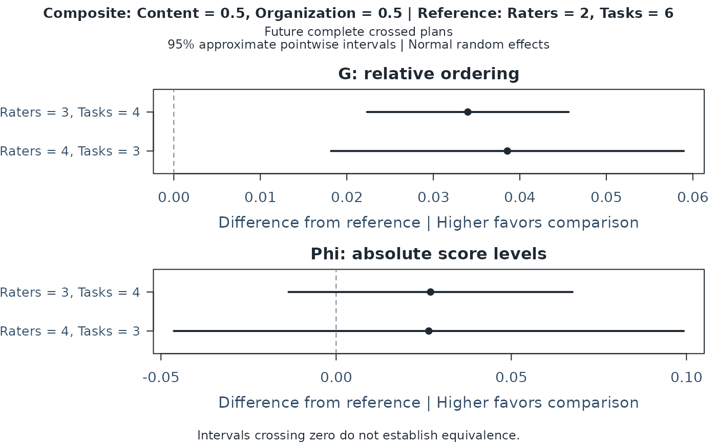
Use this comparison when choosing between plans specified before inspecting their estimates. For example, compare two raters and six tasks with three raters and four tasks. A positive G/Phi difference favors the comparison plan; a negative SEM difference favors it. An interval containing zero means the direction is uncertain, not that the plans are equivalent. Equal rating counts do not establish equal examinee burden or cost.

The current scope is two common random facets, complete balanced ANOVA or identifiable incomplete crossed MINQUE(0), and future complete crossed plans. Persons and both facets are sampled from their stated populations. The source assignments are held fixed and must preserve the random-effect distributions. One-facet, nested, fixed-facet, nonnormal-robust and informative-missingness intervals are not provided. Ordinal score labels alone do not justify normal effects. Incomplete source designs can have much weaker information than complete designs with the same numbers of observed levels.

The method uses raw estimated components in the Gaussian covariance of quadratic-form estimates, then the delta method for paired differences and a normal critical value. It uses the gradient of the difference, not a sum of independent marginal variances. For a complete source design this agrees with mean-square variances 2 * MS^2 / df. These are approximate intervals, not exact finite-sample guarantees. Small facet pools, uneven assignments and estimates near boundaries can impair the approximation. In a bounded assessment, a skewed-effect condition reduced nominal 95% coverage to about 92%; this method must not be described as distribution robust.

Negative components are retained and flagged. No components, differences or interval endpoints are clipped. An unavailable point projection, boundary derivative or nonpositive estimated difference variance leaves that interval unavailable with a reason. Identical plans have an exact zero difference when their point projections are available. Component and sampling-covariance diagnostics do not establish model fit or interval accuracy.

Intervals are pointwise for each prespecified comparison. They do not support choosing the largest observed improvement, simultaneous claims over all rows, or comparisons between adaptively selected score weights. SEM is measurement error in score units; SE here is sampling uncertainty in the difference.

Point projections are recomputed from the stored G-study using current rules; no G-study is refitted and x is not modified. The G-study must retain its analyzed data. For incomplete sources, covariance computation processes blocks of rows to avoid a full observation-by-observation matrix; its running time is still quadratic in the number of observed ratings.

Examples

# Fictional continuous ratings: two common random facets, two score components.
set.seed(24)
ratings <- expand.grid(Person = 1:40, Rater = 1:8, Task = 1:6)
ratings$Content <- ratings$Organization <- 0
sources <- list("Person", "Rater", "Task", c("Person", "Rater"),
  c("Person", "Task"), c("Rater", "Task"), c("Person", "Rater", "Task"))
for (source in sources) {
  group <- interaction(ratings[source], drop = TRUE)
  effects <- matrix(rnorm(2 * nlevels(group)), ncol = 2)
  ratings[c("Content", "Organization")] <-
    ratings[c("Content", "Organization")] + effects[as.integer(group), ]
}
g <- mfrm_multivariate_gstudy(ratings, c("Content", "Organization"))
d <- mfrm_multivariate_d_study(g,
  data.frame(Raters = c(2, 3, 4), Tasks = c(6, 4, 3)),
  weights = c(Content = .5, Organization = .5))
comparison <- mfrm_multivariate_d_compare(d, reference = 1,
  assumption = "normal")
summary(comparison)
#>   Reference Scenario      Kind     Score      Metric ReferenceValue     Value
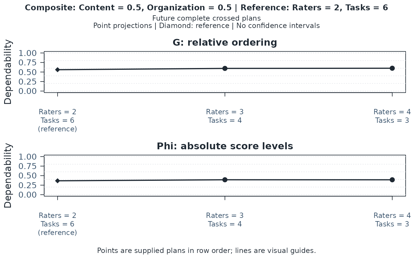
#> 1         1        2 Composite Composite           G      0.5607879 0.5947792
#> 2         1        2 Composite Composite         Phi      0.3646152 0.3915712
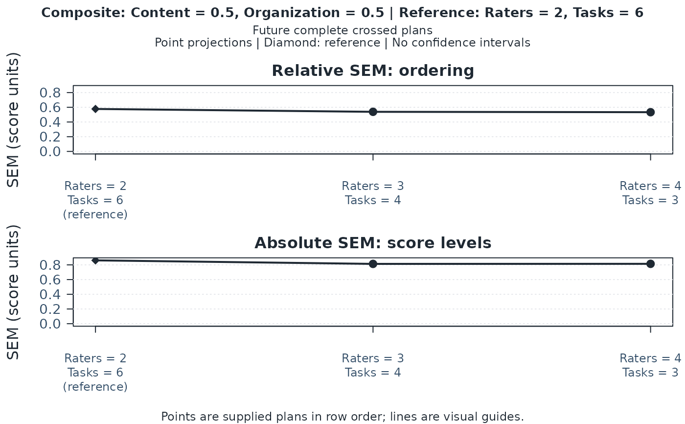
#> 3         1        2 Composite Composite RelativeSEM      0.5774748 0.5385960
#> 4         1        2 Composite Composite AbsoluteSEM      0.8613827 0.8133822
#> 5         1        3 Composite Composite           G      0.5607879 0.5993499
#> 6         1        3 Composite Composite         Phi      0.3646152 0.3910704
#> 7         1        3 Composite Composite RelativeSEM      0.5774748 0.5335039
#> 8         1        3 Composite Composite AbsoluteSEM      0.8613827 0.8142378
#>    Difference    Status          SE       Lower       Upper
#> 1  0.03399130 Available 0.005947269  0.02233487  0.04564774
#> 2  0.02695599 Available 0.020683397 -0.01358272  0.06749470
#> 3 -0.03887873 Available 0.006955045 -0.05251036 -0.02524709
#> 4 -0.04800055 Available 0.038102461 -0.12268000  0.02667890
#> 5  0.03856203 Available 0.010405112  0.01816839  0.05895568
#> 6  0.02645516 Available 0.037138595 -0.04633515  0.09924547
#> 7 -0.04397091 Available 0.011934932 -0.06736295 -0.02057887
#> 8 -0.04714496 Available 0.066016840 -0.17653559  0.08224567
plot(comparison) # G/Phi for each plan, including the reference.

plot(comparison, type = "sem")

plot(comparison, view = "differences") # Paired difference intervals.

Usage

Arguments

Value

Details

See also

Examples