Exploring person, rater, and task attributes • mfrmr

An assessment team wants to describe its raters’ backgrounds before planning training. Do groups summarize different combinations of experience, workload, and training? Would those descriptions change with the number of groups, feature weights, or plausible replacements for unrecorded attributes?

This example follows that question from a feature table to a comparison of partitions. It uses 120 fictional raters, not observations from an assessment program. No true groups are planted. Successful execution does not establish that these features, imputation models, or groups are appropriate for your raters. The groups describe backgrounds; they do not measure rater quality, severity, or ability, and do not identify which training will be effective. Later sections add separate person and task attributes, link all three classifications to a sparse assignment roster, and explain the roles of feature selection and PCA.

These APIs are available from version 0.2.4. Install the optional cluster and mice packages to run the entire example.

Choose attributes and their meaning

Use one row per rater, rather than repeating attributes for every rating. Keep identifiers separate from features. Select variables for the question before examining which choices produce attractive groups.

Column	Meaning and coding	Role here
`ExperienceYears`	Completed years of rating experience; numeric	Feature
`AnnualRatings`	Number of responses rated in the previous year; numeric	Feature
`Specialty`	Main subject area; unordered factor	Feature
`TrainingLevel`	Highest completed training stage; ordered factor	Feature
`Certified`	Holds the relevant certification; logical	Feature
`WorkshopHours`	Hours of workshops attended in the previous year; numeric	Auxiliary imputation predictor
`MentoringYears`	Years in a formal mentoring role; undefined without that role	Reviewed, then excluded from the all-rater feature set

library(mfrmr)
set.seed(20260921)
n <- 120L
raters <- data.frame(
  Rater = sprintf("R%03d", seq_len(n)),
  ExperienceYears = sample(0:30, n, replace = TRUE),
  AnnualRatings = round(exp(rnorm(n, log(250), 0.6))),
  Specialty = factor(sample(c("Language", "Science", "Social science"),
                            n, replace = TRUE)),
  TrainingLevel = ordered(sample(c("Introductory", "Intermediate", "Advanced"),
                                 n, replace = TRUE),
                          levels = c("Introductory", "Intermediate", "Advanced")),
  Certified = sample(c(FALSE, TRUE), n, replace = TRUE),
  WorkshopHours = sample(0:80, n, replace = TRUE)
)
has_mentoring_role <- sample(c(FALSE, TRUE), n, replace = TRUE, prob = c(.7, .3))
raters$MentoringYears <- ifelse(has_mentoring_role,
  pmin(raters$ExperienceYears, sample(0:10, n, replace = TRUE)), NA_real_)

# Introduce unrecorded values only after generating the fictional attributes.
feature_names <- c("ExperienceYears", "AnnualRatings", "Specialty",
                   "TrainingLevel", "Certified")
missing_counts <- c(12L, 18L, 6L, 10L, 10L)
for (j in seq_along(feature_names)) {
  raters[[feature_names[j]]][sample.int(n, missing_counts[j])] <- NA
}
head(raters)
#>   Rater ExperienceYears AnnualRatings      Specialty TrainingLevel Certified
#> 1  R001              17           545       Language      Advanced      TRUE
#> 2  R002               1           440       Language  Intermediate     FALSE
#> 3  R003              13           186        Science      Advanced      TRUE
#> 4  R004               7            NA Social science  Introductory     FALSE
#> 5  R005              21           255 Social science      Advanced     FALSE
#> 6  R006               2           150       Language  Intermediate        NA
#>   WorkshopHours MentoringYears
#> 1            27             NA
#> 2             0             NA
#> 3            66             10
#> 4            30             NA
#> 5            60             NA
#> 6            21             NA

The Gower distance calculation accommodates these mixed types. Numeric features use their observed ranges. Ordered levels use ordered integer codes, so the declared order and the spacing implicit in that coding matter. Logical features treat both matches (FALSE/FALSE and TRUE/TRUE) alike. Certification is therefore not coded as a special presence-only attribute. Equal feature weights are a starting choice; correlated or redundant attributes can still receive too much combined influence. A highly unusual numeric value can also change its feature’s range and hence other raters’ distances.

Distinguish unrecorded and undefined values

Here a missing mentoring duration means that the attribute does not apply. It is not a duration waiting to be estimated. A duration of zero would instead mean an applicable mentoring role with no completed years.

all_features <- c(feature_names, "MentoringYears")
initial <- mfrm_features(raters, "Rater", all_features)
reasons <- initial$missing
reasons$Reason <- ifelse(reasons$Feature == "MentoringYears",
                        "Not applicable: no mentoring role", "Not recorded")
review <- mfrm_features(raters, "Rater", all_features, reasons)
summary(review)
#>           Feature             Type Observed Missing Distinct
#> 1 ExperienceYears          Numeric      108      12       30
#> 2   AnnualRatings          Numeric      102      18       94
#> 3       Specialty          Nominal      114       6        3
#> 4   TrainingLevel          Ordinal      110      10        3
#> 5       Certified Symmetric binary      110      10        2
#> 6  MentoringYears          Numeric       33      87       11
table(review$missing$Reason)
#> 
#> Not applicable: no mentoring role                      Not recorded 
#>                                87                                56

The target is a description of all raters. Requiring a mentoring duration would exclude nonmentors. We therefore leave it out of the selected features and the imputation predictors, retaining the original review. A separate analysis confined to mentors would address a different population.

selected_reasons <- subset(review$missing, Feature %in% feature_names)
features <- mfrm_features(raters, "Rater", feature_names, selected_reasons)
features$feature_summary
#>           Feature             Type Observed Missing Distinct
#> 1 ExperienceYears          Numeric      108      12       30
#> 2   AnnualRatings          Numeric      102      18       94
#> 3       Specialty          Nominal      114       6        3
#> 4   TrainingLevel          Ordinal      110      10        3
#> 5       Certified Symmetric binary      110      10        2
table(features$row_summary$Complete)
#> 
#> FALSE  TRUE 
#>    48    72

mfrm_cluster_pam(features, k = 3) would stop on the remaining missing values. Explicit missing = "omit" is available, but selects complete raters and changes the population being described. It does not correct missing-data bias.

Fit an explicit imputation model

Only cells reviewed as unrecorded are eligible here. The fictional omissions were introduced at random; in an actual program, an explanation based on the data collection process is needed. Missingness reasons alone do not identify a statistical missingness mechanism. Unobserved-value-dependent nonresponse requires additional sensitivity assumptions.

The mice documentation describes the methods and predictor controls used below. WorkshopHours can help predict unrecorded attributes without becoming a clustering feature. The identifier is neither imputed nor used to predict other variables.

eligible <- subset(features$missing, Reason == "Not recorded")
imputation_data <- raters[c("Rater", feature_names, "WorkshopHours")]
where <- matrix(FALSE, nrow(imputation_data), ncol(imputation_data),
                dimnames = dimnames(imputation_data))
where[cbind(match(eligible$ID, imputation_data$Rater),
            match(eligible$Feature, names(imputation_data)))] <- TRUE
methods <- mice::make.method(imputation_data, where = where)
methods[feature_names] <- c("pmm", "pmm", "polyreg", "polr", "logreg")
methods["Rater"] <- ""
predictors <- mice::make.predictorMatrix(imputation_data)
predictors[, "Rater"] <- 0
predictors["Rater", ] <- 0
model <- mice::mice(imputation_data, m = 5, maxit = 5,
  method = methods, predictorMatrix = predictors, where = where,
  seed = 724, printFlag = FALSE)
model$loggedEvents
#> NULL
plot(model, c("ExperienceYears", "AnnualRatings"), layout = c(2, 2))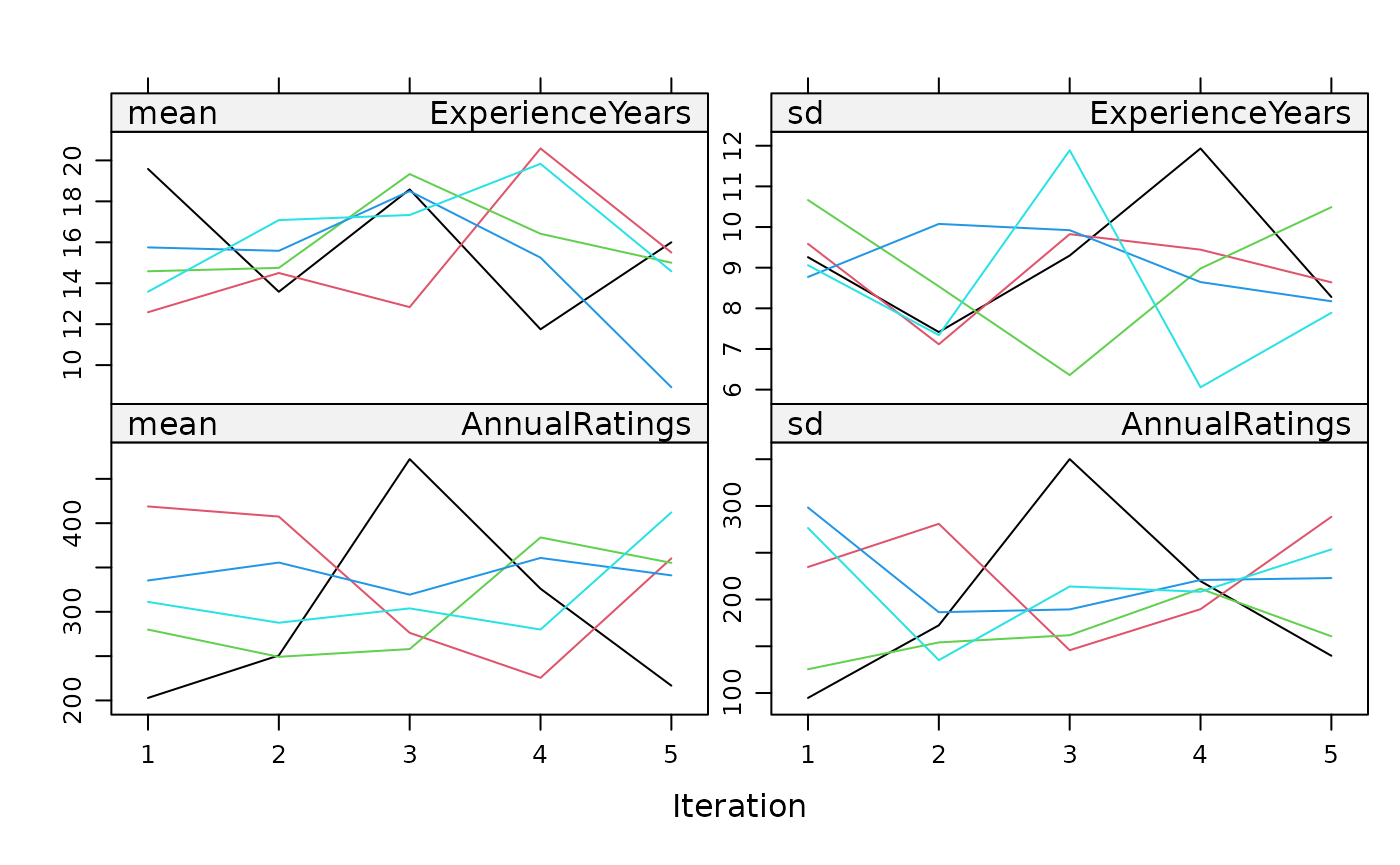

Imputation-chain means and standard deviations across iterations for experience years and annual rating workload. These traces help review mixing; they do not establish that the imputation model is appropriate.

Five imputations and five iterations keep this executable example short; they are not an adequacy recommendation. The plot shows the mean and standard deviation of imputed values along each chain for two numeric features. Persistent drift or differences between chains call for investigation; overlapping lines in this short example do not establish convergence. Inspect logged events, chain behavior, observed versus imputed distributions, and substantive plausibility. A lack of logged events does not establish convergence or a suitable model. mfrm_cluster_imputed() checks consistency of the data, not these assumptions.

Describe groups and compare choices

Reuse the same fitted imputation model for every setting. Changing the imputations as well as the weights would change two things at once.

experience_weights <- setNames(rep(1, length(feature_names)), feature_names)
experience_weights["ExperienceYears"] <- 3
analyses <- list(
  TwoGroups = mfrm_cluster_imputed(features, model, eligible, k = 2),
  ThreeGroups = mfrm_cluster_imputed(features, model, eligible, k = 3),
  ExperienceWeighted = mfrm_cluster_imputed(features, model, eligible, k = 3,
                                          weights = experience_weights)
)
comparison <- mfrm_cluster_compare(analyses)
comparison$analysis_summary
#>              Analysis Method Linkage Imputation K Features Included Excluded
#> 1           TwoGroups    PAM    <NA>          1 2        5      120        0
#> 2           TwoGroups    PAM    <NA>          2 2        5      120        0
#> 3           TwoGroups    PAM    <NA>          3 2        5      120        0
#> 4           TwoGroups    PAM    <NA>          4 2        5      120        0
#> 5           TwoGroups    PAM    <NA>          5 2        5      120        0
#> 6         ThreeGroups    PAM    <NA>          1 3        5      120        0
#> 7         ThreeGroups    PAM    <NA>          2 3        5      120        0
#> 8         ThreeGroups    PAM    <NA>          3 3        5      120        0
#> 9         ThreeGroups    PAM    <NA>          4 3        5      120        0
#> 10        ThreeGroups    PAM    <NA>          5 3        5      120        0
#> 11 ExperienceWeighted    PAM    <NA>          1 3        5      120        0
#> 12 ExperienceWeighted    PAM    <NA>          2 3        5      120        0
#> 13 ExperienceWeighted    PAM    <NA>          3 3        5      120        0
#> 14 ExperienceWeighted    PAM    <NA>          4 3        5      120        0
#> 15 ExperienceWeighted    PAM    <NA>          5 3        5      120        0
#>    MinGroupSize MaxGroupSize MeanSilhouette Distance          Space Scaling
#> 1            51           69      0.2841483    Gower Mixed features   Range
#> 2            52           68      0.2584725    Gower Mixed features   Range
#> 3            56           64      0.2681527    Gower Mixed features   Range
#> 4            47           73      0.2338481    Gower Mixed features   Range
#> 5            57           63      0.2578823    Gower Mixed features   Range
#> 6            37           43      0.2526199    Gower Mixed features   Range
#> 7            37           42      0.2813456    Gower Mixed features   Range
#> 8            37           42      0.2628245    Gower Mixed features   Range
#> 9            36           44      0.2401655    Gower Mixed features   Range
#> 10           39           42      0.2521256    Gower Mixed features   Range
#> 11           32           47      0.1915956    Gower Mixed features   Range
#> 12           36           45      0.1964619    Gower Mixed features   Range
#> 13           34           47      0.2290490    Gower Mixed features   Range
#> 14           36           46      0.2250179    Gower Mixed features   Range
#> 15           36           47      0.2256632    Gower Mixed features   Range
#>    Components
#> 1          NA
#> 2          NA
#> 3          NA
#> 4          NA
#> 5          NA
#> 6          NA
#> 7          NA
#> 8          NA
#> 9          NA
#> 10         NA
#> 11         NA
#> 12         NA
#> 13         NA
#> 14         NA
#> 15         NA
summary(comparison)
#>         First             Second Partitions Included Pairs MeanChangedFraction
#> 1   TwoGroups        ThreeGroups          5      120  7140           0.3199160
#> 2   TwoGroups ExperienceWeighted          5      120  7140           0.3930812
#> 3 ThreeGroups ExperienceWeighted          5      120  7140           0.3063866
#>   MinChangedFraction MaxChangedFraction MeanAdjustedRand
#> 1          0.2715686          0.3567227        0.3621596
#> 2          0.2397759          0.4521008        0.2171547
#> 3          0.1901961          0.4263305        0.3080772
weight_effect <- subset(comparison$comparison_summary,
  First == "ThreeGroups" & Second == "ExperienceWeighted")

MeanChangedFraction describes the fraction of rater pairs whose together/apart status changes between settings, averaged over the supplied imputations. The minimum and maximum show its range. The individual rows in comparison$comparisons retain every imputation, including split/join counts and adjusted Rand indices. An adjusted Rand index of one indicates identical partitions, allowing arbitrary group numbering. Neither high agreement nor a large silhouette proves that the groups are meaningful. Silhouettes under different weights use different distances and should not automatically select the weights.

In this fictional example, keeping three groups and raising the experience weight from one to three changes the together/apart status of 30.6% of rater pairs on average across imputations. Thus, the selected weights materially affect this particular description; presenting a single partition would conceal that dependence. This percentage concerns pairs, not the percentage of raters assigned to a different numbered group. It is not evidence about an actual assessment program.

Also inspect MinGroupSize. A rare category can produce a very small group, and repeated profiles can give high separation values. A high overall silhouette can coexist with these conditions.

Compare feature selections

Does including annual rating workload change the background groups? Hold the raters, group count, method, and imputation model fixed, and remove AnnualRatings from the clustering features. Select the corresponding eligible cells rather than passing cells for an unselected feature.

background_names <- setdiff(feature_names, "AnnualRatings")
background_features <- mfrm_features(raters, "Rater", background_names,
  subset(selected_reasons, Feature %in% background_names))
background_only <- mfrm_cluster_imputed(background_features, model,
  subset(eligible, Feature %in% background_names), k = 3)
feature_comparison <- mfrm_cluster_compare(list(
  WithWorkload = analyses$ThreeGroups, WithoutWorkload = background_only))
feature_comparison$analysis_summary
#>           Analysis Method Linkage Imputation K Features Included Excluded
#> 1     WithWorkload    PAM    <NA>          1 3        5      120        0
#> 2     WithWorkload    PAM    <NA>          2 3        5      120        0
#> 3     WithWorkload    PAM    <NA>          3 3        5      120        0
#> 4     WithWorkload    PAM    <NA>          4 3        5      120        0
#> 5     WithWorkload    PAM    <NA>          5 3        5      120        0
#> 6  WithoutWorkload    PAM    <NA>          1 3        4      120        0
#> 7  WithoutWorkload    PAM    <NA>          2 3        4      120        0
#> 8  WithoutWorkload    PAM    <NA>          3 3        4      120        0
#> 9  WithoutWorkload    PAM    <NA>          4 3        4      120        0
#> 10 WithoutWorkload    PAM    <NA>          5 3        4      120        0
#>    MinGroupSize MaxGroupSize MeanSilhouette Distance          Space Scaling
#> 1            37           43      0.2526199    Gower Mixed features   Range
#> 2            37           42      0.2813456    Gower Mixed features   Range
#> 3            37           42      0.2628245    Gower Mixed features   Range
#> 4            36           44      0.2401655    Gower Mixed features   Range
#> 5            39           42      0.2521256    Gower Mixed features   Range
#> 6            38           42      0.3037361    Gower Mixed features   Range
#> 7            38           42      0.2797405    Gower Mixed features   Range
#> 8            35           49      0.2571784    Gower Mixed features   Range
#> 9            36           44      0.2639301    Gower Mixed features   Range
#> 10           37           42      0.2940627    Gower Mixed features   Range
#>    Components
#> 1          NA
#> 2          NA
#> 3          NA
#> 4          NA
#> 5          NA
#> 6          NA
#> 7          NA
#> 8          NA
#> 9          NA
#> 10         NA
feature_comparison$weights
#>          Analysis         Feature Weight
#> 1    WithWorkload ExperienceYears      1
#> 2    WithWorkload   AnnualRatings      1
#> 3    WithWorkload       Specialty      1
#> 4    WithWorkload   TrainingLevel      1
#> 5    WithWorkload       Certified      1
#> 6 WithoutWorkload ExperienceYears      1
#> 7 WithoutWorkload       Specialty      1
#> 8 WithoutWorkload   TrainingLevel      1
#> 9 WithoutWorkload       Certified      1
summary(feature_comparison)
#>          First          Second Partitions Included Pairs MeanChangedFraction
#> 1 WithWorkload WithoutWorkload          5      120  7140           0.2570308
#>   MinChangedFraction MaxChangedFraction MeanAdjustedRand
#> 1                  0           0.327591         0.418318

Here, removing workload changes the together/apart status of 25.7% of rater pairs on average across the five imputations. This measures the description’s dependence on including workload, not whether workload should be excluded. The Features column records each analysis’s feature count; weights lists only its selected features. Silhouettes now use different distances and cannot automatically choose a feature set.

Workload remains in the imputation model, so this does not examine removing it as a predictor of missing attributes. Different feature selections must reuse the same fitted mids object, and stored completed values are checked against the corresponding imputation. A selection containing only complete attributes can use its empty missing table as impute; it retains a partition for every completion for comparison purposes.

The included entities must match across all results. With missing = "omit", removing an incomplete feature may admit additional raters, in which case the comparison stops. Define and report a common cohort before fitting if that is the intended question; the API does not silently intersect samples.

Interpret the retained profiles

Inspect the actual profiles before attaching interpretations to the groups:

one_completion <- analyses$ThreeGroups$analyses[[1]]
one_completion$profiles$numeric
#>   Cluster         Feature  N      Mean Median         SD
#> 1       1 ExperienceYears 37  16.83784   17.0   9.601833
#> 2       1   AnnualRatings 37 233.18919  171.0 141.312663
#> 3       2 ExperienceYears 40  17.57500   21.0   7.944963
#> 4       2   AnnualRatings 40 357.15000  277.5 259.475758
#> 5       3 ExperienceYears 43  16.46512   17.0   9.074687
#> 6       3   AnnualRatings 43 341.02326  309.0 181.776614
subset(one_completion$profiles$categorical, Feature == "TrainingLevel")
#>    Cluster       Feature        Level  N Proportion
#> 4        1 TrainingLevel Introductory 24  0.6486486
#> 5        1 TrainingLevel Intermediate  9  0.2432432
#> 6        1 TrainingLevel     Advanced  4  0.1081081
#> 12       2 TrainingLevel Introductory  9  0.2250000
#> 13       2 TrainingLevel Intermediate 19  0.4750000
#> 14       2 TrainingLevel     Advanced 12  0.3000000
#> 20       3 TrainingLevel Introductory 10  0.2325581
#> 21       3 TrainingLevel Intermediate  7  0.1627907
#> 22       3 TrainingLevel     Advanced 26  0.6046512
head(one_completion$membership)
#>     ID Cluster Medoid  Silhouette
#> 1 R001       1  FALSE  0.23012013
#> 2 R002       2  FALSE -0.06900752
#> 3 R003       2  FALSE  0.11688238
#> 4 R004       3  FALSE  0.33805884
#> 5 R005       3  FALSE  0.47966587
#> 6 R006       1  FALSE  0.37930314
analyses$ThreeGroups$co_membership[1:5, 1:5]
#>      R001 R002 R003 R004 R005
#> R001  1.0  0.2  0.2  0.0  0.0
#> R002  0.2  1.0  0.4  0.4  0.4
#> R003  0.2  0.4  1.0  0.0  0.0
#> R004  0.0  0.4  0.0  1.0  1.0
#> R005  0.0  0.4  0.0  1.0  1.0

These profiles describe one completion, not an average cluster or a final assignment. Group numbers can change across completions. The co_membership matrix instead records how often each pair is grouped together across all imputations. For example, 0.8 means four of the five completions, conditional on this model and these settings. It is not an 80% probability of a true shared class. Numeric ranges are recalculated within each completion; their changes also contribute to sensitivity.

The workflow answers whether proposed background descriptions depend strongly on the supplied choices. It supplies no automatic preferred group count, consensus assignment, resampling stability, Rubin-pooled inference, or imputation of rating responses. Before using groups to make decisions about raters, establish that the attributes and proposed use address the intended question and assess the consequences with appropriate evidence.

Read separation, feature profiles, and imputation sensitivity

The silhouette plot shows which raters fit their assigned group less clearly under the selected distances. Negative widths warrant examining the rater’s profile and nearby groups; high widths do not establish useful or stable types. The dashed line is the overall mean. Raters excluded from clustering have no width; their IDs remain in the returned plot data.

plot(one_completion)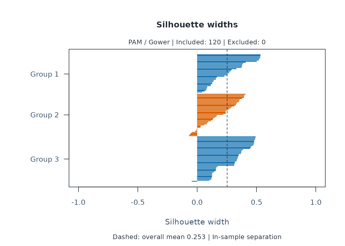

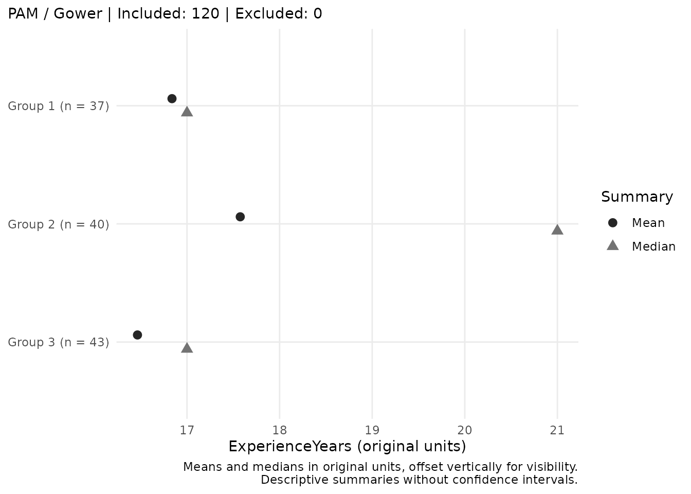
Rater silhouette widths grouped by the descriptive partition in one completion. The dashed line is the overall mean; negative widths indicate profiles to inspect, not poor rater quality.

Inspect one feature at a time so that its units and categories remain clear. Numeric profiles show means and medians in original units, without confidence intervals. Categorical profiles show proportions within each group, preserving the order of training levels. These are descriptions of this completion only.

plot(one_completion, type = "profile", feature = "ExperienceYears")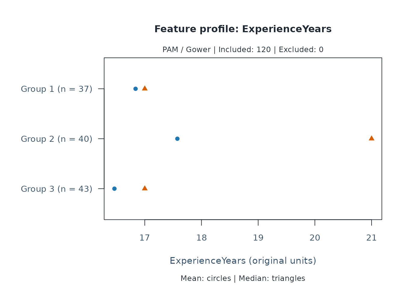

Experience in years summarized by descriptive rater group, with means and medians in the original units and no confidence intervals.

plot(one_completion, type = "profile", feature = "TrainingLevel")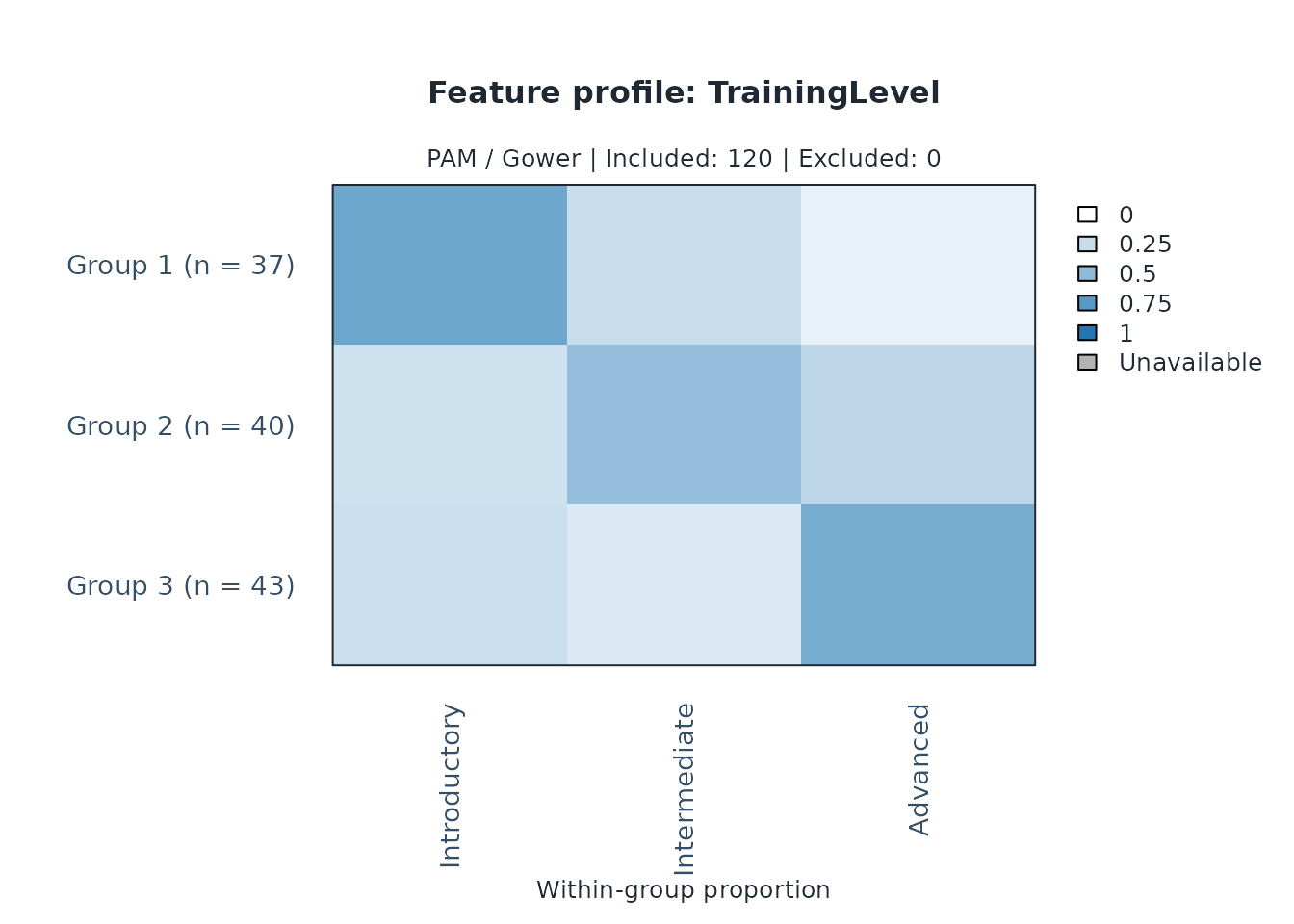

Proportions of ordered training levels within each descriptive rater group. These profiles describe one imputed table, not effects of training.

The development version also offers dedicated ggplot conversion for these saved summaries. For example, remove the heading while keeping the original units, group sizes and interpretation note:

if (requireNamespace("ggplot2", quietly = TRUE)) {
  profile_figure <- as_ggplot(one_completion, type = "profile",
    feature = "ExperienceYears", preset = "monochrome") +
    ggplot2::labs(title = NULL)
  print(profile_figure)
}

Use as_ggplot(one_completion) for the silhouette view, retaining negative widths and the saved overall-mean line. Use the profile call with feature = "TrainingLevel" for a categorical heatmap, including unused levels in their original order. The default and component = "table" keep the full view; categorical profiles also accept component = "matrix". Means and medians are descriptive, not effect estimates or interval bounds. The slight vertical offsets improve visibility without changing the values. Saved summaries and excluded IDs remain available through plot_data().

The next heatmap asks which pairs remain together across imputations. For readability, this view explicitly selects the first 20 IDs in the input table; it does not recluster them, change the denominator, or represent the remaining pairs. Omit ids to display all raters. By default, ID labels are hidden above 50 displayed entities; the data are never sampled automatically.

plot(analyses$ThreeGroups, ids = raters$Rater[1:20])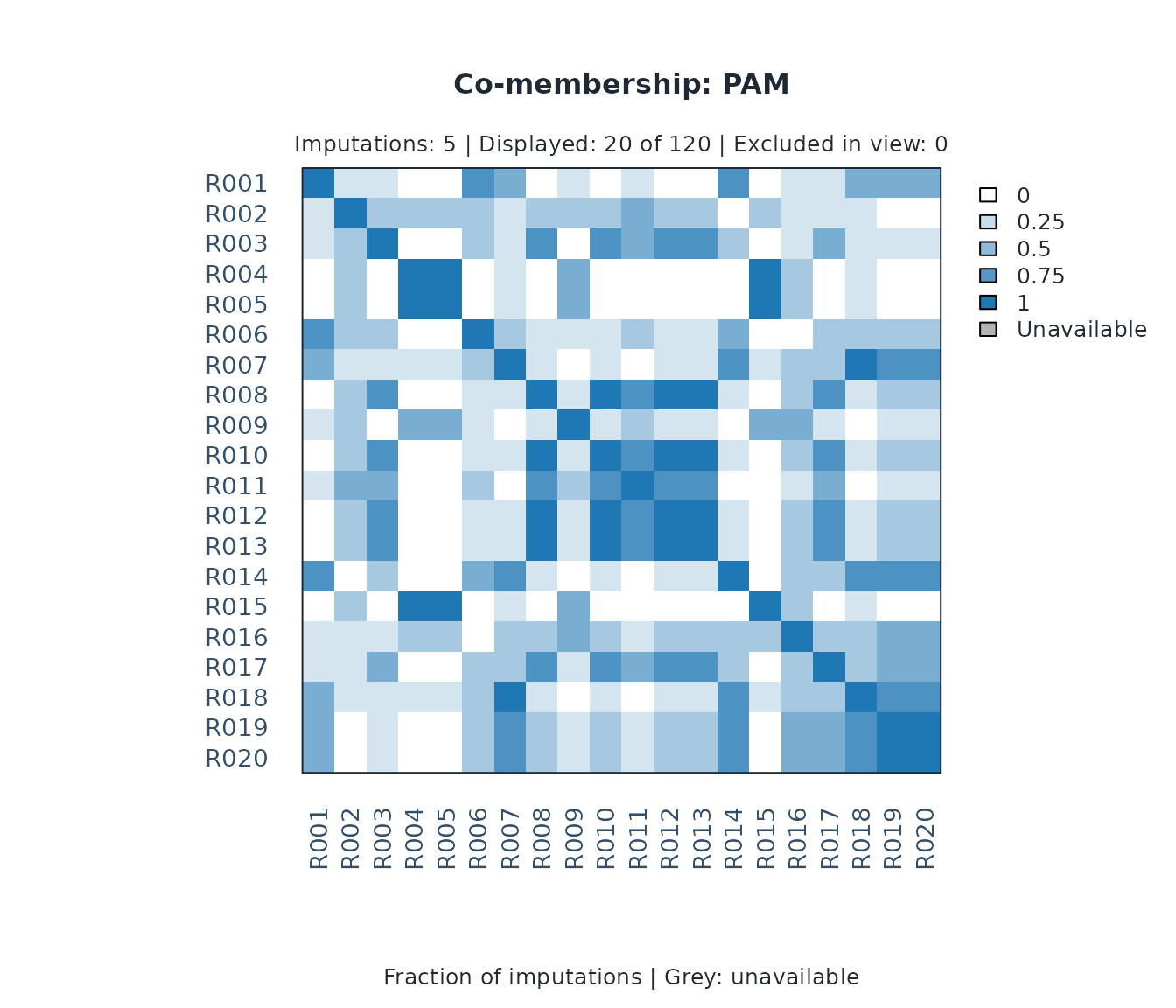

Pairwise co-membership proportions across imputations for the first twenty rater IDs. The scale runs from zero to one; unavailable pairs are grey. These proportions are imputation sensitivity, not sampling stability.

The colour scale always runs from zero to one. Grey denotes unavailable pairs involving excluded raters, not pairs that never share a group. Rows retain the requested ID order. The map does not infer a consensus partition or a hierarchy, and it does not measure stability under new samples of raters.

For a custom figure, extract the same values without drawing or refitting:

view <- plot(analyses$ThreeGroups, ids = raters$Rater[1:5], draw = FALSE)
plot_data(view)$matrix
#>      R001 R002 R003 R004 R005
#> R001  1.0  0.2  0.2  0.0  0.0
#> R002  0.2  1.0  0.4  0.4  0.4
#> R003  0.2  0.4  1.0  0.0  0.0
#> R004  0.0  0.4  0.0  1.0  1.0
#> R005  0.0  0.4  0.0  1.0  1.0

The development version also converts this same five-ID view to ggplot:

if (requireNamespace("ggplot2", quietly = TRUE)) {
  co_membership_figure <- as_ggplot(view, component = "matrix") +
    ggplot2::labs(title = NULL)
  print(co_membership_figure)
}

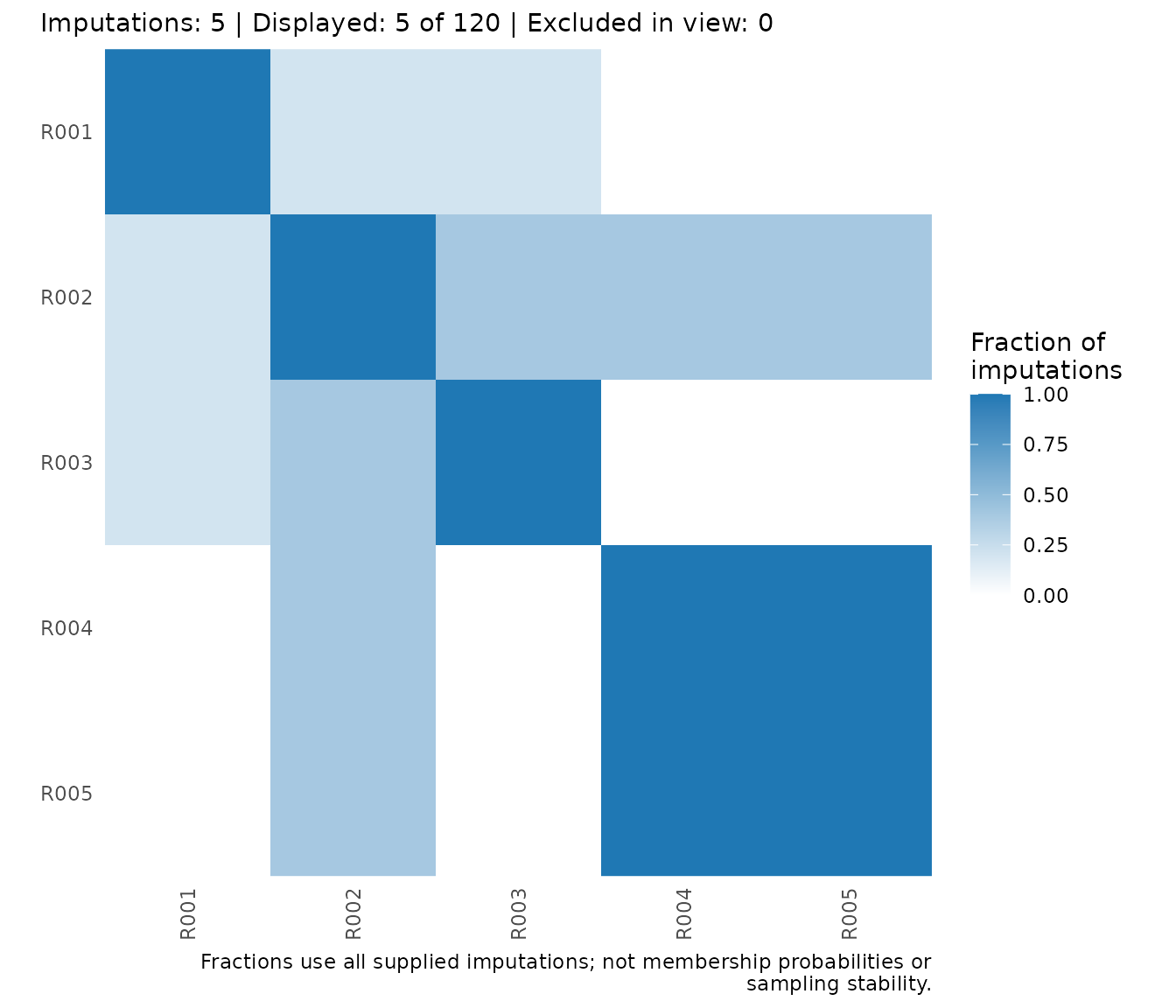
$Co-membership fractions for the five selected rater IDs, in the saved order on both axes. The scale is fixed from zero to one; crosses mark unavailable cells, if any. Values use all supplied imputations and do not measure sampling stability.$

The default and component = "matrix" retain the same complete heatmap. For a new selection, use as_ggplot(analyses$ThreeGroups, ids = ...) or create another saved plot with plot(..., draw = FALSE). A saved view keeps its preset and label choice even after session options change. Grey cells also carry crosses, so unavailable pairs remain distinct from zero in monochrome. plot_data(co_membership_figure) retains the matrix, selected IDs, excluded IDs and number of imputations. Hiding headings with ggplot2::labs() does not remove those records or change the meaning of the fractions.

Compare PAM with a hierarchy

A hierarchy asks which groups merge as dissimilarity increases. Fit it separately from PAM: mfrm_cluster_hierarchical() uses average linkage (the mean of all cross-group Gower dissimilarities) or complete linkage (their maximum). The same feature types, weights, and missingness rules apply. Choose the group count explicitly; a tree does not automatically identify it.

For multiply imputed features, reuse the same model and eligible cells. This holds the completed tables fixed while changing the grouping method.

average <- mfrm_cluster_imputed(features, model, eligible, k = 3,
  method = "hierarchical", linkage = "average")
complete <- mfrm_cluster_imputed(features, model, eligible, k = 3,
  method = "hierarchical", linkage = "complete")
method_comparison <- mfrm_cluster_compare(list(
  PAM = analyses$ThreeGroups, Average = average, Complete = complete))
method_comparison$analysis_summary
#>    Analysis       Method  Linkage Imputation K Features Included Excluded
#> 1       PAM          PAM     <NA>          1 3        5      120        0
#> 2       PAM          PAM     <NA>          2 3        5      120        0
#> 3       PAM          PAM     <NA>          3 3        5      120        0
#> 4       PAM          PAM     <NA>          4 3        5      120        0
#> 5       PAM          PAM     <NA>          5 3        5      120        0
#> 6   Average Hierarchical  average          1 3        5      120        0
#> 7   Average Hierarchical  average          2 3        5      120        0
#> 8   Average Hierarchical  average          3 3        5      120        0
#> 9   Average Hierarchical  average          4 3        5      120        0
#> 10  Average Hierarchical  average          5 3        5      120        0
#> 11 Complete Hierarchical complete          1 3        5      120        0
#> 12 Complete Hierarchical complete          2 3        5      120        0
#> 13 Complete Hierarchical complete          3 3        5      120        0
#> 14 Complete Hierarchical complete          4 3        5      120        0
#> 15 Complete Hierarchical complete          5 3        5      120        0
#>    MinGroupSize MaxGroupSize MeanSilhouette Distance          Space Scaling
#> 1            37           43      0.2526199    Gower Mixed features   Range
#> 2            37           42      0.2813456    Gower Mixed features   Range
#> 3            37           42      0.2628245    Gower Mixed features   Range
#> 4            36           44      0.2401655    Gower Mixed features   Range
#> 5            39           42      0.2521256    Gower Mixed features   Range
#> 6            32           48      0.3452806    Gower Mixed features   Range
#> 7            35           43      0.3409728    Gower Mixed features   Range
#> 8            33           46      0.3469410    Gower Mixed features   Range
#> 9            34           46      0.3398082    Gower Mixed features   Range
#> 10           33           45      0.3389007    Gower Mixed features   Range
#> 11           32           48      0.3452806    Gower Mixed features   Range
#> 12           35           43      0.3409728    Gower Mixed features   Range
#> 13           20           54      0.3053761    Gower Mixed features   Range
#> 14           20           67      0.2888587    Gower Mixed features   Range
#> 15           38           42      0.3861780    Gower Mixed features   Range
#>    Components
#> 1          NA
#> 2          NA
#> 3          NA
#> 4          NA
#> 5          NA
#> 6          NA
#> 7          NA
#> 8          NA
#> 9          NA
#> 10         NA
#> 11         NA
#> 12         NA
#> 13         NA
#> 14         NA
#> 15         NA
summary(method_comparison)
#>     First   Second Partitions Included Pairs MeanChangedFraction
#> 1     PAM  Average          5      120  7140           0.3474230
#> 2     PAM Complete          5      120  7140           0.3309244
#> 3 Average Complete          5      120  7140           0.1263025
#>   MinChangedFraction MaxChangedFraction MeanAdjustedRand
#> 1          0.2756303          0.3703081        0.2158120
#> 2          0.2516807          0.3962185        0.2673826
#> 3          0.0000000          0.2676471        0.7239888

The comparison identifies methods and linkages, alongside group sizes and separation. As before, pair-change summaries describe sensitivity to the supplied choices; they do not select a preferred algorithm or establish true rater types. Substantively different profiles or very small groups deserve inspection even when the overall pair agreement is high.

plot(average$analyses[[1]])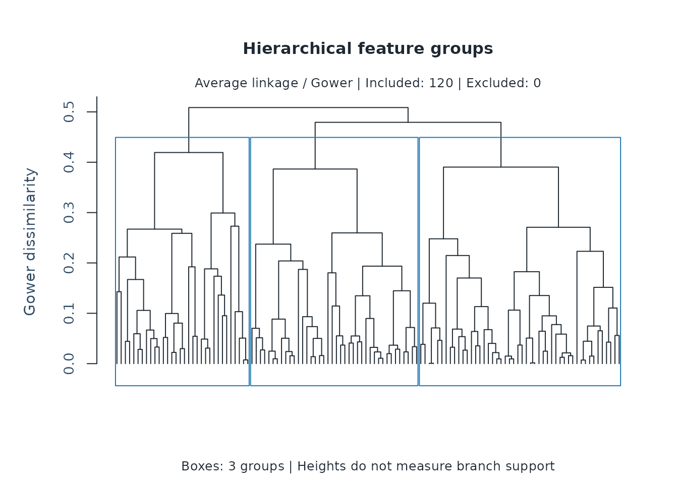

Average-linkage hierarchy from Gower dissimilarities in one completed rater-feature table. Boxes mark three groups; all 120 raters are included. Heights are dissimilarities, not significance or branch support.

This is the full tree for one completion, with boxes marking its three groups. The 120 raters are all included; ID labels are hidden by default above 50 entities. For a smaller cohort, labels appear automatically. Use plot_data(plot(average$analyses[[1]], draw = FALSE))$table to inspect IDs and memberships in leaf order. Excluded raters retain unavailable memberships but have no leaves. No entities are sampled to draw the tree.

In the development version, as_ggplot(average$analyses[[1]]) converts this same saved tree with its group boxes, leaf order and merge heights. The default and component = "tree" retain the full view; use plot_data() for the membership table. Conversion does not refit, recut or combine trees across completions. Add ggplot2::labs(title = NULL, subtitle = NULL) to omit headings, while retaining the caption about what heights mean.

Merge heights are linkage dissimilarities, not significance levels or branch support. Tied distances can produce alternative trees; the group cut uses merge order, so a unique horizontal cutting height may not exist. Inspect each completion’s profiles with type = "profile" or silhouettes with type = "silhouette". plot(average) displays pairwise co-membership across imputations; it does not combine the trees into a consensus hierarchy.

How this relates to MFRM rater-type research

Clustering has been used alongside MFRM, with both hierarchical and nonhierarchical methods. In writing assessment, Eckes (2012), Operational Rater Types in Writing Assessment, clustered MFRM rater-by-criterion bias estimates using hierarchical Ward clustering, also checking complete and average linkage solutions. In music performance assessment, Wesolowski (2019), Predicting Operational Rater-Type Classifications Using Rasch Measurement Theory and Random Forests, reported nonhierarchical k-means clustering of 29 differential rater functioning indices, followed by prediction of the resulting labels.

Those analyses ask about patterns of rating behaviour. This tutorial instead groups external backgrounds such as experience and specialty. Its Gower distances accommodate the selected mix of variable types, and PAM produces a partition rather than a hierarchy. The separate hierarchical API uses average or complete linkage. Ward’s variance criterion requires appropriate Euclidean geometry; this Gower interface does not define a Euclidean conversion and does not offer Ward clustering (see Murtagh and Legendre, 2014). The cited studies do not validate the present attributes, weights, imputation model, or PAM groups, and do not establish that one method is preferable for all uses. Grouping estimated MFRM effects would additionally require consideration of their measurement uncertainty and comparability. The present external-feature API does not propagate that uncertainty.

Link separately grouped persons, raters, and tasks

An assessment team may also ask whether different kinds of persons and tasks are represented across its rater groups. Keep three feature tables, with one row per person, rater, or task, and a separate rating table containing their IDs. The tables can have different numbers and types of features. Clustering the joined rating rows would repeat attributes according to assignment frequency and answer a different question about rating events.

Table	Example features	Unit classified
Persons	Years of language study, preparation hours, instruction mode	One person
Raters	Experience, workload, specialty, training, certification	One rater
Tasks	Time limit, word limit, response format	One task

The following extends the fictional example with 240 persons and 12 tasks. It uses the existing rater partition from one completed table only to illustrate joining by ID. The other two tables have no missing attributes. The group counts are illustrative choices, not estimated numbers of types.

set.seed(7241)
persons <- data.frame(
  Person = sprintf("P%03d", 1:240),
  LanguageStudyYears = sample(0:15, 240, replace = TRUE),
  PreparationHours = round(exp(rnorm(240, log(20), 0.5))),
  InstructionMode = factor(sample(c("Classroom", "Online", "Hybrid"),
                                  240, replace = TRUE)))
tasks <- data.frame(
  Task = sprintf("T%02d", 1:12),
  TimeLimitMinutes = sample(c(10, 20, 30), 12, replace = TRUE),
  WordLimit = sample(c(100, 200, 400), 12, replace = TRUE),
  ResponseFormat = factor(rep(c("Summary", "Argument", "Explanation"), 4)))
person_groups <- mfrm_cluster_pam(mfrm_features(persons, "Person",
  c("LanguageStudyYears", "PreparationHours", "InstructionMode")), k = 3)
task_groups <- mfrm_cluster_pam(mfrm_features(tasks, "Task",
  c("TimeLimitMinutes", "WordLimit", "ResponseFormat")), k = 3)

Record the planned assignments before collecting scores. Here each person receives three distinct tasks and each performance is assigned two distinct raters. The full Person-by-Rater-by-Task cross-product is not the assignment roster. Random scores below are placeholders for demonstrating coverage; they provide no evidence about achievement, rater effects, or model fit.

assignments <- do.call(rbind, lapply(persons$Person, function(id) {
  do.call(rbind, lapply(sample(tasks$Task, 3), function(task) {
    data.frame(Person = id, Rater = sample(raters$Rater, 2), Task = task)
  }))
}))
ratings <- assignments
ratings$Score <- sample(1:4, nrow(ratings), replace = TRUE)
ratings$Score[sample(nrow(ratings), 72)] <- NA_integer_
rating_review <- describe_mfrm_data(ratings, person = "Person",
  facets = c("Rater", "Task"), score = "Score",
  rating_min = 1, rating_max = 4, keep_original = TRUE,
  include_agreement = FALSE, expected_design = assignments)
rating_review$structural_missingness$summary
#>     Status ExpectedCells ObservedCells MatchedCells MissingExpectedCells
#> 1 declared          1440          1368         1368                   72
#>   UnexpectedObservedCells CoverageRate ExpectedOnlyPersons UnexpectedPersons
#> 1                       0         0.95                   0                 0
rating_review$design_connectivity
#>               Basis Facet PersonNodes FacetLevelNodes Edges Components
#> 1          observed Rater         240             120  1352          1
#> 2          observed  Task         240              12   715          1
#> 3 declared_expected Rater         240             120  1422          1
#> 4 declared_expected  Task         240              12   720          1
#>   LargestComponentPersons LargestComponentLevels LargestComponentPercent
#> 1                     240                    120                     100
#> 2                     240                     12                     100
#> 3                     240                    120                     100
#> 4                     240                     12                     100
#>   Connected
#> 1      TRUE
#> 2      TRUE
#> 3      TRUE
#> 4      TRUE

There are 1,440 assigned cells out of 345,600 possible combinations, and 72 assigned scores are absent. Assignment coverage is therefore 95%, even though fewer than 0.5% of all combinations were assigned. Neither a zero score nor an imputed score is inserted into unassigned cells. With actual data, supply the original roster: reconstructing it from observed scores would conceal missing assigned ratings.

Start from the assignment roster so that even an entirely absent rating row remains in the denominator. This example has one score per Person-Rater-Task key; check uniqueness before joining. For repeated occasions, include the occasion in the key. Attach the three independently obtained group labels by ID with match(); row position in a feature table is not an ID. The check stops this illustration if an ID is unknown or an entity has no classification. In an analysis allowing omitted entities, report their unclassified ratings separately rather than silently dropping them.

rating_key <- c("Person", "Rater", "Task")
stopifnot(!anyDuplicated(assignments[rating_key]),
          !anyDuplicated(ratings[rating_key]))
labeled <- merge(assignments, ratings, by = rating_key,
                 all.x = TRUE, sort = FALSE)
labeled$PersonGroup <- person_groups$membership$Cluster[
  match(labeled$Person, person_groups$membership$ID)]
labeled$RaterGroup <- one_completion$membership$Cluster[
  match(labeled$Rater, one_completion$membership$ID)]
labeled$TaskGroup <- task_groups$membership$Cluster[
  match(labeled$Task, task_groups$membership$ID)]
group_columns <- c("PersonGroup", "RaterGroup", "TaskGroup")
stopifnot(!anyNA(labeled[group_columns]))
for (column in group_columns) labeled[[column]] <- factor(labeled[[column]], 1:3)
labeled$Assigned <- 1L
labeled$Observed <- as.integer(!is.na(labeled$Score))
planned_counts <- xtabs(Assigned ~ PersonGroup + RaterGroup + TaskGroup,
                        data = labeled)
observed_counts <- xtabs(Observed ~ PersonGroup + RaterGroup + TaskGroup,
                         data = labeled)
group_coverage <- as.data.frame(planned_counts, responseName = "Assigned")
group_coverage$Observed <- as.vector(observed_counts)
group_coverage$Coverage <- ifelse(group_coverage$Assigned > 0,
  group_coverage$Observed / group_coverage$Assigned, NA_real_)
group_coverage
#>    PersonGroup RaterGroup TaskGroup Assigned Observed  Coverage
#> 1            1          1         1       49       46 0.9387755
#> 2            2          1         1       51       48 0.9411765
#> 3            3          1         1       55       52 0.9454545
#> 4            1          2         1       50       47 0.9400000
#> 5            2          2         1       46       42 0.9130435
#> 6            3          2         1       43       37 0.8604651
#> 7            1          3         1       65       61 0.9384615
#> 8            2          3         1       59       55 0.9322034
#> 9            3          3         1       56       54 0.9642857
#> 10           1          1         2       45       43 0.9555556
#> 11           2          1         2       30       29 0.9666667
#> 12           3          1         2       53       53 1.0000000
#> 13           1          2         2       52       51 0.9807692
#> 14           2          2         2       64       62 0.9687500
#> 15           3          2         2       64       60 0.9375000
#> 16           1          3         2       63       59 0.9365079
#> 17           2          3         2       62       59 0.9516129
#> 18           3          3         2       65       64 0.9846154
#> 19           1          1         3       44       40 0.9090909
#> 20           2          1         3       39       39 1.0000000
#> 21           3          1         3       51       49 0.9607843
#> 22           1          2         3       59       57 0.9661017
#> 23           2          2         3       66       61 0.9242424
#> 24           3          2         3       44       42 0.9545455
#> 25           1          3         3       53       49 0.9245283
#> 26           2          3         3       63       62 0.9841270
#> 27           3          3         3       49       47 0.9591837

This table answers which group combinations were assigned and how many of their scores were recorded. A combination with no assignments has unavailable coverage, not zero coverage. Counts reflect the assignment design; they do not demonstrate associations between traits or differences in rating quality. Ratings share persons, raters, and tasks, so an ordinary independent-row test of group differences would not account for this dependence. Raw score means also confound person composition, rater severity, and task difficulty. Such comparisons need an appropriate measurement model and sufficient overlap, rather than treating the group labels as established latent classes.

If attributes are imputed for several facets, each imputation model must respect its unit of analysis and relevant dependencies. The current API analyzes one entity table at a time; it does not fit a joint cross-facet imputation model or pool group-by-group rating effects. Pairing the first completion of independently fitted person and rater models does not establish a valid joint imputation. Nor can numeric group labels be matched across completions without addressing label changes and membership uncertainty.

Distinguish sparse assignment from missing attributes

Four situations require different decisions:

Situation	Example	What to retain or review
Unassigned rating	A rater was never scheduled to score a performance	Original assignment roster; no invented observation
Missing assigned rating	A scheduled score was not submitted	Assigned denominator, absence reason, observed overlap
Unrecorded external attribute	Training hours were not recorded	Eligible cells, predictors, imputation assumptions
Undefined external attribute	Mentoring years for someone with no mentoring role	Meaning of the attribute; not an ordinary imputation target

Sparseness describes how much of a design is observed and how those observations connect. MCAR means that missingness does not depend on the observed or missing values. MAR allows dependence on observed values, but not on missing values after conditioning on the observed information. MNAR allows additional dependence on the missing values. Planned allocation does not automatically imply MCAR: assignment may depend on recorded proficiency or on information absent from the analysis. A missingness rate or diagnostic test alone cannot establish MAR. See Rubin (1976), Inference and Missing Data for the conditions for ignoring a missingness process in inference.

Inspect both planned and observed connectivity, per-level support, and coverage within relevant subgroups. Connected Person-facet graphs do not by themselves establish identification of a complete model, especially with interactions, or adequate precision. In a simulation of sparse MFRM designs, Wind and Ge (2021) found that detecting differential rater functioning depended on the linking design, not merely on having incomplete ratings. Their findings do not give a universal acceptable missingness percentage. Imputing external attributes does not add observed links or resolve confounding between disconnected rating blocks. Grouping noisy estimated effects from sparse data may also reflect differences in precision, which this feature API does not model.

Many features, k-means, and PCA

More columns are not necessarily more useful information. Repeated measures of one attribute can dominate a distance through their combined weight; unrelated columns can obscure the differences of interest. Steinley and Brusco (2008) examined variable selection for clustering and found that non-informative variables and their distributions affected performance. Choose features and their substantive domains before choosing weights. For example, equal total weight for a domain containing ten features and one containing two requires different per-feature weights. This is a substantive choice, not an automatic correction for correlations. The comparison API supports both positive feature weights and different selections on the same entities, as illustrated above. Choosing features to maximize an attractive grouping still requires separate validation; the comparison does not automate feature selection.

PCA and k-means answer different questions. PCA represents variation in numeric features with orthogonal continuous components. K-means partitions entities to minimize within-group squared Euclidean distances to centroids. Ding and He (2004), Principal Component Analysis and Effective K-means Clustering describe their relationship through a continuous relaxation of discrete cluster membership. This does not make ordinary PCA and discrete clustering equivalent, or establish that the first two PCs recover useful groups.

For a fixed numeric input, retaining all nonzero PC scores without further rescaling preserves its Euclidean distances. Truncating components changes those distances and may remove low-variance separation as well as noise. Standardizing features before PCA, or whitening the scores afterwards, also changes the chosen geometry. An explained-variance threshold alone is not evidence that a clustering structure was preserved. A two-component plot is a projection, not a test for the existence of clusters.

Ordinary PCA and k-means should not receive arbitrary numeric codes for nominal categories such as specialty. Keep Gower/PAM or average/complete linkage for mixed features. For selected numeric attributes, mfrm_pca() and mfrm_cluster_kmeans() use R’s prcomp() and kmeans(). They center features and, by default, divide by sample standard deviations. Positive feature weights apply to squared Euclidean distances. The fitted transformation, original units, entity IDs and missingness accounting remain available. No automatic feature, component or group-count selection is performed.

Here the question is whether grouping experience, annual workload and workshop hours changes when those three attributes are represented by two components. The same already fitted imputation model supplies both analyses. Workshop hours remain a predictor in that model whether or not they are selected for clustering. These numeric selections answer a different question from the mixed-background groups above; specialty and training level are not numeric inputs to this PCA.

numeric_names <- c("ExperienceYears", "AnnualRatings", "WorkshopHours")
numeric_review <- mfrm_features(raters, "Rater", numeric_names)
numeric_direct <- mfrm_cluster_imputed(numeric_review, model,
  numeric_review$missing, k = 3, method = "kmeans", seed = 42)
numeric_reduced <- mfrm_cluster_imputed(numeric_review, model,
  numeric_review$missing, k = 3, method = "kmeans", components = 2, seed = 42)
numeric_comparison <- mfrm_cluster_compare(list(
  StandardizedFeatures = numeric_direct, TwoComponents = numeric_reduced))
numeric_comparison$analysis_summary
#>                Analysis  Method Linkage Imputation K Features Included Excluded
#> 1  StandardizedFeatures k-means    <NA>          1 3        3      120        0
#> 2  StandardizedFeatures k-means    <NA>          2 3        3      120        0
#> 3  StandardizedFeatures k-means    <NA>          3 3        3      120        0
#> 4  StandardizedFeatures k-means    <NA>          4 3        3      120        0
#> 5  StandardizedFeatures k-means    <NA>          5 3        3      120        0
#> 6         TwoComponents k-means    <NA>          1 3        3      120        0
#> 7         TwoComponents k-means    <NA>          2 3        3      120        0
#> 8         TwoComponents k-means    <NA>          3 3        3      120        0
#> 9         TwoComponents k-means    <NA>          4 3        3      120        0
#> 10        TwoComponents k-means    <NA>          5 3        3      120        0
#>    MinGroupSize MaxGroupSize MeanSilhouette  Distance                Space
#> 1            23           55      0.2946332 Euclidean     Numeric features
#> 2            31           49      0.2921438 Euclidean     Numeric features
#> 3            30           47      0.2890823 Euclidean     Numeric features
#> 4            21           51      0.2841480 Euclidean     Numeric features
#> 5            23           53      0.2742463 Euclidean     Numeric features
#> 6            27           51      0.4118746 Euclidean Principal components
#> 7            29           50      0.4118474 Euclidean Principal components
#> 8            27           52      0.3786295 Euclidean Principal components
#> 9            34           44      0.3871943 Euclidean Principal components
#> 10           28           51      0.3811840 Euclidean Principal components
#>      Scaling Components
#> 1  Sample SD         NA
#> 2  Sample SD         NA
#> 3  Sample SD         NA
#> 4  Sample SD         NA
#> 5  Sample SD         NA
#> 6  Sample SD          2
#> 7  Sample SD          2
#> 8  Sample SD          2
#> 9  Sample SD          2
#> 10 Sample SD          2
summary(numeric_comparison)
#>                  First        Second Partitions Included Pairs
#> 1 StandardizedFeatures TwoComponents          5      120  7140
#>   MeanChangedFraction MinChangedFraction MaxChangedFraction MeanAdjustedRand
#> 1           0.1959384         0.02072829          0.3857143        0.5701576

Read Space, Scaling and Components before comparing the partitions. ChangedFraction measures changed together/apart pairs, allowing arbitrary renumbering of clusters. Different component counts change distances, so silhouette widths do not provide a common-scale test that one analysis is better. The default 25 random starts and fixed seed make this execution reproducible, but do not prove a global optimum. Assess another seed separately if initialization sensitivity matters.

first_numeric <- numeric_reduced$analyses[[1]]
summary(first_numeric$pca)
#>   Component  Variance Proportion Cumulative Retained
#> 1       PC1 1.1248279  0.3749426  0.3749426     TRUE
#> 2       PC2 0.9952593  0.3317531  0.7066957     TRUE
#> 3       PC3 0.8799128  0.2933043  1.0000000    FALSE
first_numeric$pca$loadings
#>                        PC1          PC2
#> ExperienceYears -0.4657154  0.761955112
#> AnnualRatings    0.5411158  0.647598960
#> WorkshopHours   -0.7002163 -0.006324086
plot(first_numeric$pca)  # The full explained-variance table, including omitted PCs.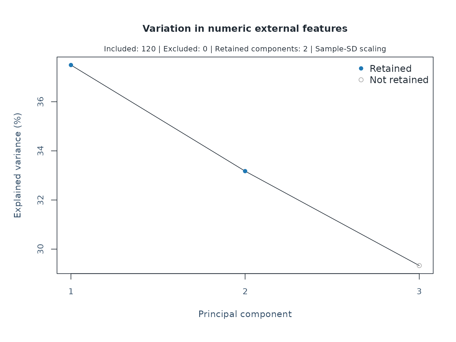

Explained-variance scree plot for numeric rater features in one completion. Filled points identify retained components and open points identify omitted components.

plot(first_numeric$pca, type = "scores", groups = first_numeric, labels = FALSE)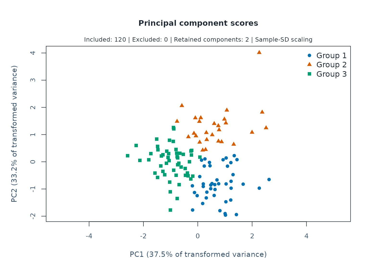

Scores on the first two principal components, with descriptive k-means groups distinguished by colour and point shape. This projection is not a latent ability or rater-quality scale.

plot(first_numeric$pca, type = "loadings", components = 1)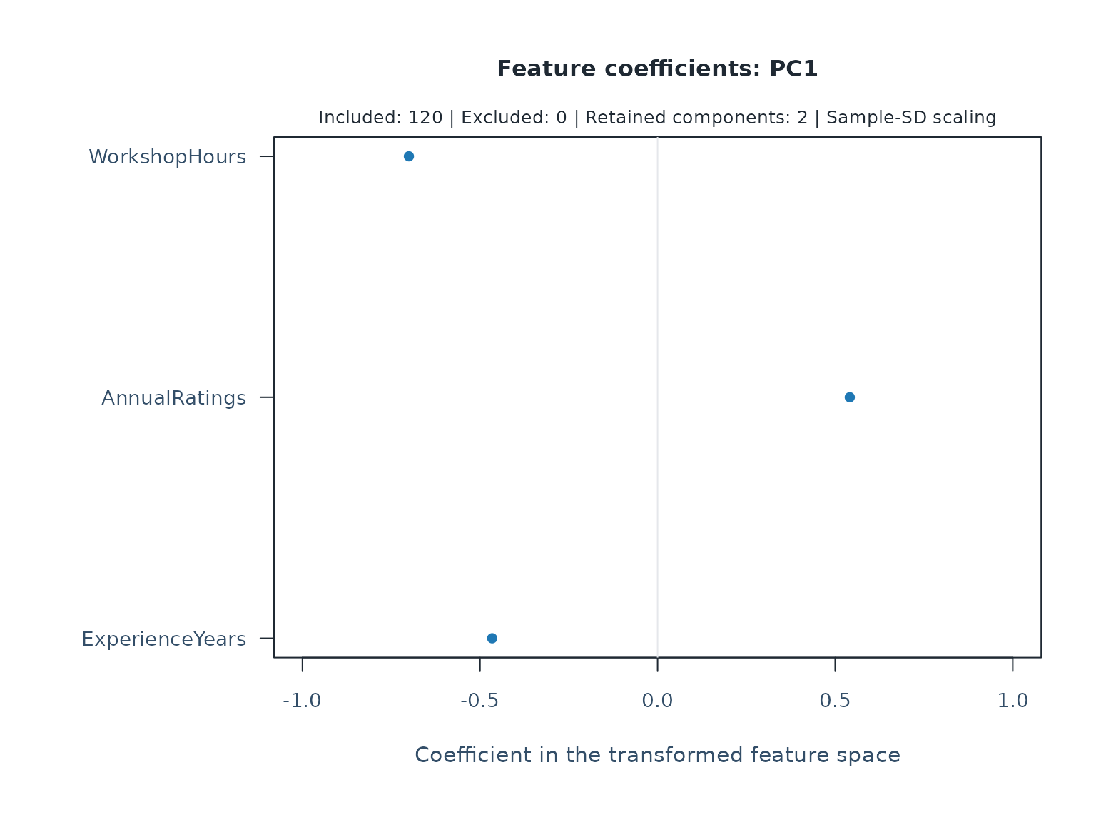

First-component loadings for the transformed numeric rater features. Their signs are arbitrary and the coefficients are not original-unit correlations.

plot(first_numeric, type = "profile", feature = "ExperienceYears")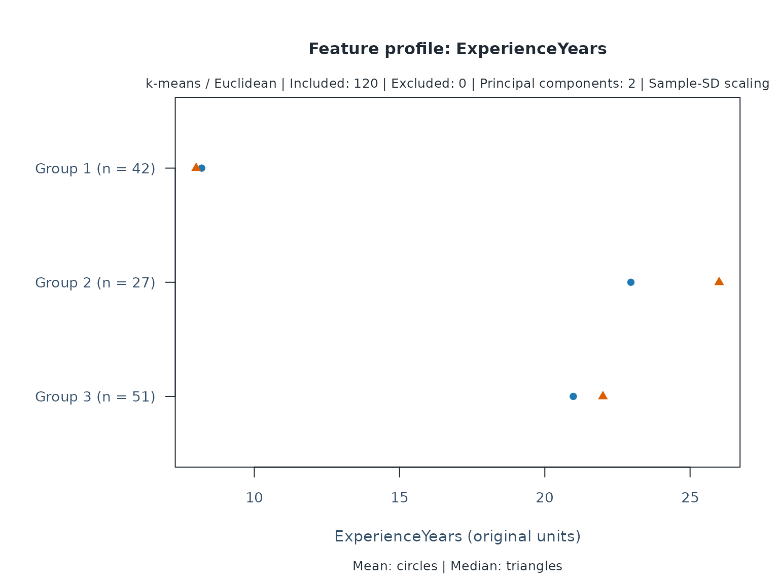

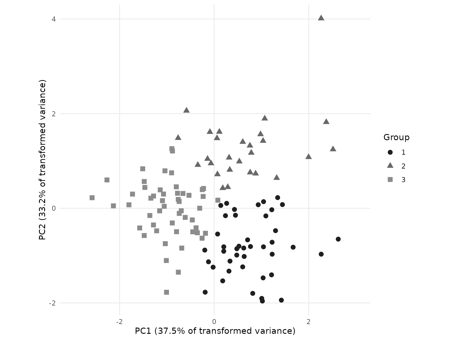
Experience in years summarized by the k-means groups fitted in the retained principal-component space. The original-unit profile describes this completion only.

The first-completion score plot annotates a two-dimensional projection with that completion’s group labels. Colour and point shape distinguish groups; preset = "monochrome" retains the shapes. Shapes repeat after six groups, so inspect plot_data() for IDs and encodings in crowded views. Filled/open scree points distinguish retained/omitted components. Loadings are coefficients in the transformed feature space, not correlations in original units. Their signs are arbitrary. Inspect the original-unit profiles to explain what distinguishes the groups. No view establishes ability, severity, rater quality or an effect of training.

Every completion retains its own centering, standard deviations and PCA basis. The comparison pairs the same completions, while allowing these transformations to change as imputed values change. It compares partitions; it does not average PCA scores, loadings or arbitrary group numbers, and it does not Rubin-pool inference. These functions impute no rating scores.

For an already complete numeric table, use mfrm_cluster_kmeans(review, k=3) directly. To inspect and retain a specific reduction, fit pca <- mfrm_pca(review, components=2) and then mfrm_cluster_kmeans(pca, k=3). Passing a PCA object uses its scores exactly, without further standardization, range scaling or whitening. Save that PCA and its grouping together. plot() and mfrm_cluster_compare() reuse saved results; changing features, component counts, weights or seeds requires the corresponding new analysis. mfrmr_output_guide("features") lists the dedicated output routes. Use summary() for partition comparisons, and plot() or plot_data() for fitted PCA and grouping views.

In the development version, as_ggplot() has dedicated conversions for PCA scree, scores and loadings. The scores view keeps the selected components, equal axis units and the saved group colours and shapes. Only included entities are drawn; excluded IDs and the feature transformation remain in plot_data(). This example shows the same first completion used above:

if (requireNamespace("ggplot2", quietly = TRUE)) {
  numeric_figure <- as_ggplot(first_numeric$pca, type = "scores",
    groups = first_numeric, labels = FALSE, preset = "monochrome") +
    ggplot2::labs(title = NULL, subtitle = NULL)
  print(numeric_figure)
  plot_data(numeric_figure)$components
}

Scores on the first two external-feature principal components for one completed feature dataset. K-means groups use grayscale colours and different point shapes. Headings and entity labels are omitted; the saved data still identify the completion's transformation and excluded entities.

#> [1] 1 2

Use type = "scree" for explained-variance percentages and type = "loadings" for coefficients in the transformed feature space. The default and explicit component = "table" keep the same complete view. For already saved plot payloads, as_ggplot() uses their saved preset and label choice; set those choices when making the payload. A change of heading does not change the analysis. Saved dendrograms also have dedicated conversion as described above. Imputation co-membership also has dedicated conversion as described above. Silhouettes and numeric/categorical profiles also have dedicated conversion. All these views retain their saved summaries; use plot_data() for further custom graphics.

Reopen an analysis without repeating imputation or clustering

Keep the complete imputed analysis to retain every completion, its PCA basis and partition, the fitted imputation model, and the co-membership summary. A saved plot view also retains the selected display settings. The example uses a temporary file; choose a permanent path to continue in a later session.

feature_file <- tempfile(fileext = ".rds")
feature_view <- plot(first_numeric$pca, type = "scores", groups = first_numeric,
  labels = FALSE, preset = "monochrome", draw = FALSE)
saveRDS(list(analysis = numeric_reduced, view = feature_view), feature_file)
saved_features <- readRDS(feature_file)
summary(saved_features$analysis)  # Review all completions.
#>   Imputation Included Excluded MeanSilhouette
#> 1          1      120        0      0.4118746
#> 2          2      120        0      0.4118474
#> 3          3      120        0      0.3786295
#> 4          4      120        0      0.3871943
#> 5          5      120        0      0.3811840
plot_data(saved_features$view)    # Inspect this first-completion view.
#> $table
#>       ID         PC1          PC2 Cluster
#> 1   R001  0.87634235  0.733479843       2
#> 2   R002  2.26336239 -0.969851454       1
#> 3   R003 -1.03369410 -0.747832237       3
#> 4   R004  0.31282340 -1.328179610       1
#> 5   R005 -1.09352767  0.160883647       3
#> 6   R006  0.81518883 -1.798216746       1
#> 7   R007 -0.80140952  0.453468531       3
#> 8   R008  0.76120416  0.756505024       2
#> 9   R009 -0.89540056  1.259120586       3
#> 10  R010  0.18137681  0.425836679       2
#> 11  R011 -1.57542512 -0.415843745       3
#> 12  R012  0.28759049  0.447101980       2
#> 13  R013 -2.13099007  0.051149385       3
#> 14  R014 -1.07150264  0.300792002       3
#> 15  R015 -0.79592341 -0.495630537       3
#> 16  R016  1.06924913  1.895353435       2
#> 17  R017  0.31489989  1.070143764       2
#> 18  R018 -0.61241972 -0.192779197       3
#> 19  R019  0.47751548 -0.989263769       1
#> 20  R020  0.62555830 -0.840354187       1
#> 21  R021  0.42955400 -0.024721049       1
#> 22  R022 -0.53234977  0.274006878       3
#> 23  R023 -0.19051687 -1.773355422       1
#> 24  R024  1.04252312 -0.814539579       1
#> 25  R025 -0.68597143 -0.840850895       3
#> 26  R026  0.23869502 -0.156548442       1
#> 27  R027 -0.88601398 -0.310073756       3
#> 28  R028  2.37019247  1.820995805       2
#> 29  R029 -0.34587530  0.915407863       2
#> 30  R030  0.78440032  1.172184883       2
#> 31  R031  1.03495506 -1.470972831       1
#> 32  R032 -1.36041835 -0.152873822       3
#> 33  R033  0.32944281  0.813178588       2
#> 34  R034  1.00602464 -1.904821679       1
#> 35  R035 -0.25114660  0.394754494       3
#> 36  R036 -0.45311017 -0.497935040       3
#> 37  R037 -0.75945359  0.187692339       3
#> 38  R038  0.47899202 -0.854941661       1
#> 39  R039  0.05965514  1.480370614       2
#> 40  R040 -1.14162145  0.389001993       3
#> 41  R041  0.60452459  1.401849050       2
#> 42  R042  1.04430511  0.139651084       1
#> 43  R043 -0.76240240  1.484568234       2
#> 44  R044 -1.15311864 -0.054295210       3
#> 45  R045  0.75634109  1.324083832       2
#> 46  R046  1.09306279 -0.161649766       1
#> 47  R047  0.07235875 -0.544703673       1
#> 48  R048 -0.69654559 -0.053008749       3
#> 49  R049 -0.02245593 -1.244927976       1
#> 50  R050  0.93170546  0.074777829       1
#> 51  R051 -1.80249480  0.073327838       3
#> 52  R052 -0.19848423 -0.883757420       1
#> 53  R053 -1.00783264 -1.774789239       3
#> 54  R054 -1.51150814  0.834154237       3
#> 55  R055 -1.72709711  0.299724379       3
#> 56  R056  0.52351515 -0.801657065       1
#> 57  R057 -1.21682284 -0.476835993       3
#> 58  R058 -0.38239696 -0.413306564       3
#> 59  R059 -0.22486385  0.418509730       3
#> 60  R060  0.45056336 -0.147045448       1
#> 61  R061 -1.04102070  0.791468885       3
#> 62  R062  1.21344568 -1.406872487       1
#> 63  R063 -0.35565333 -0.517461973       3
#> 64  R064  2.51360935  1.245062557       2
#> 65  R065  0.13952449  0.059760071       1
#> 66  R066 -0.65968317  0.312749190       3
#> 67  R067  1.44350811  0.077931116       1
#> 68  R068  0.20186672 -0.908138211       1
#> 69  R069  1.22672484 -0.970702572       1
#> 70  R070  0.33452532 -1.116727288       1
#> 71  R071 -0.06746429  0.949576911       2
#> 72  R072 -0.46291132 -0.246601301       3
#> 73  R073  0.98033514  1.563890667       2
#> 74  R074 -0.90099583  0.748909655       3
#> 75  R075 -1.28376361 -0.352464006       3
#> 76  R076 -0.73869784 -0.109109064       3
#> 77  R077 -1.46579073  0.440324713       3
#> 78  R078  1.21837159 -0.030687999       1
#> 79  R079 -1.33886639  0.213566646       3
#> 80  R080  0.63469555 -1.018505422       1
#> 81  R081  2.62371250 -0.652139161       1
#> 82  R082  0.70701336 -0.667332623       1
#> 83  R083 -0.58567728  2.061376558       2
#> 84  R084  1.03418087  1.423846740       2
#> 85  R085 -0.12051389 -1.131091144       1
#> 86  R086 -0.88207509  1.210837203       3
#> 87  R087 -2.26769787  0.599146619       3
#> 88  R088  0.20287691 -0.814432355       1
#> 89  R089  1.32192543  0.640423109       2
#> 90  R090  1.01944279 -1.960693706       1
#> 91  R091 -0.08992824  1.611686791       2
#> 92  R092  0.26373044  0.104604625       1
#> 93  R093 -0.18444850 -0.528358653       3
#> 94  R094  1.99671866  1.080652348       2
#> 95  R095 -1.01211899 -1.104277393       3
#> 96  R096 -1.05661892  0.042188288       3
#> 97  R097  1.22487338 -0.717554314       1
#> 98  R098  0.18022881 -1.534138400       1
#> 99  R099  0.06919171  0.717506076       2
#> 100 R100 -0.77556573  0.317924051       3
#> 101 R101 -0.75745768 -1.350288915       3
#> 102 R102  1.34228980  0.225511381       1
#> 103 R103 -1.47969295 -0.575642893       3
#> 104 R104  0.60310652 -1.238183726       1
#> 105 R105 -2.58197881  0.223020060       3
#> 106 R106  1.66996020 -0.822511261       1
#> 107 R107 -1.28224072  0.258722755       3
#> 108 R108  0.53167765  0.988932604       2
#> 109 R109 -0.25556529 -0.632475987       3
#> 110 R110 -0.14063557  1.043879695       2
#> 111 R111  0.07741817  0.170911976       3
#> 112 R112  0.10968210  1.615779522       2
#> 113 R113 -1.47919119  0.566102169       3
#> 114 R114  1.29771483 -0.473164766       1
#> 115 R115 -0.74054930  0.144039195       3
#> 116 R116  2.26200482  4.011819347       2
#> 117 R117 -0.23315983  0.249806850       3
#> 118 R118  1.42118981 -1.941785212       1
#> 119 R119 -0.30659021  0.001105732       3
#> 120 R120  0.76787906 -0.808235062       1
#> 
#> $components
#> [1] 1 2
#> 
#> $encoding
#>   Cluster  Colour Shape
#> 1       1 #1F1F1F    16
#> 2       2 #686868    17
#> 3       3 #8C8C8C    15
#> 
#> $transformation
#>           Feature  Center    Divisor WeightFactor
#> 1 ExperienceYears  16.950   8.824003            1
#> 2   AnnualRatings 313.150 206.610975            1
#> 3   WorkshopHours  35.975  23.124603            1
#> 
#> $weights
#> ExperienceYears   AnnualRatings   WorkshopHours 
#>               1               1               1 
#> 
#> $scale
#> [1] TRUE
#> 
#> $excluded_ids
#> character(0)
#> 
#> $title
#> [1] "Principal component scores"
#> 
#> $subtitle
#> [1] "Included: 120 | Excluded: 0 | Retained components: 2 | Sample-SD scaling"
#> 
#> $xlab
#> [1] "PC1 (37.5% of transformed variance)"
#> 
#> $ylab
#> [1] "PC2 (33.2% of transformed variance)"
#> 
#> $labels
#> [1] FALSE
#> 
#> $preset
#> [1] "monochrome"
#> 
#> $plot_name
#> [1] "feature_pca_scores"
#> 
#> $legend
#> [1] label     role      aesthetic value    
#> <0 rows> (or 0-length row.names)
#> 
#> $reference_lines
#> [1] axis     value    label    linetype role    
#> <0 rows> (or 0-length row.names)
if (requireNamespace("ggplot2", quietly = TRUE)) {
  saved_figure <- as_ggplot(saved_features$view)
}

Changing a session plotting option does not restyle a saved view. Create a new view from the saved analysis to change its preset; changing the analysis settings requires a new analysis. These feature results use their own summary(), plot() and plot_data() methods. They are separate from mfrm_results() and from the pooled response-score intervals described in vignette("mfrmr-response-imputation"). Saved feature files retain identifiers and original attributes, so review what they contain before sharing them.

Plan for the size of the analysis

K-means can explicitly omit silhouettes with silhouette = FALSE, avoiding their quadratic distance matrix. Those silhouettes are unavailable, not zero; profile plots and partition comparisons remain available. PCA itself uses a numeric matrix decomposition whose cost depends on both entity and feature counts. Neither option promises a universal capacity limit. The imputation co-membership matrix remains quadratic even with silhouettes disabled.

Pairwise distances require memory that grows quadratically with the number of raters. Gower/PAM and hierarchical clustering permit up to 5,000 included entities; the imputation workflow permits up to 5,000 total entities because its comparison matrix includes excluded IDs. These are input limits, not a guarantee of low memory use or acceptable run time. Multiple imputations also retain every completed analysis. Save the fitted imputation model and clustering results; mfrm_cluster_compare() reuses them without repeating the fits.

Plan for temporary distance and silhouette calculations as well as the saved result. For scale, a run with 5,000 entities and eight mixed-type features, fitting two hierarchical configurations and comparing them, used about 1.5 GiB of peak process memory on macOS arm64 with R 4.6.1. The returned comparison occupied about 3.3 MiB. Average and complete linkage gave similar memory requirements in this example. These single-run measurements include R startup and data preparation; they are not a memory bound or a prediction for other machines, features, or imputation counts. The 5,000-entity imputation workflow was not evaluated in that example.

Increasing feature count also increases distance calculations and stored profiles. A separate run with 1,000 entities and 1,000 mixed-type features, again fitting and comparing two configurations, took about six seconds per method and used approximately 400–430 MiB of peak process memory on the same platform, for PAM, average linkage, and complete linkage. This was a complete-feature workload without planted groups. It does not establish useful classification, joint performance at the largest entity and feature counts, or feasibility of a 1,000-feature imputation model. A large imputation model requires its own predictor selection and checks for information, dependence, and model fit.