Plan measurement conditions with a multivariate D-study

Would adding tasks or raters make assessment scores more dependable? Use an estimated G-study to compare specified future designs for individual score components and optional weighted composites. Each scenario reports dependability and measurement error for mean scores over common random measurement conditions, such as tasks, raters, or occasions. No model is refitted.

Usage

mfrm_multivariate_d_study(x, design_grid = NULL, weights = NULL)

# S3 method for class 'mfrm_multivariate_d_study'
print(x, ...)

# S3 method for class 'mfrm_multivariate_d_study'
summary(object, ...)

Arguments

x: A result from mfrm_multivariate_gstudy().
design_grid: A nonempty data frame with one positive integer count column per G-study facet. With the rater/task interface, use Raters and/or Tasks for the included facets. With facets, use its exact labels, for example Rater and Occasion for facets = c(Rater = "Assessor", Occasion = "Session"). The mapping is available in x$design$count_columns. Each row is one future complete balanced design preserving the G-study's crossed or nested structure. For nesting = c(Rater = "Task"), Raters means raters per task, not the total rater pool. NULL uses the G-study counts (children per parent for a nested facet) only when its retained data are complete and balanced; incomplete or unequal designs require an explicit grid. Counts need not match or exceed the G-study counts. Conditions are shared across persons and scores in every scenario.
weights: Optional named numeric vector for one composite, or a numeric matrix for several named composites. A vector must name every original score exactly once; matrix rows must name every score exactly once, and columns must have unique, nonempty composite names. Rows are matched by name, regardless of order. Every weight must be finite and each composite must have at least one nonzero weight. Signed weights allow difference scores, for example c(Content = 1, Organization = -1). Weights are used as supplied, without normalization. NULL reports original scores only. Otherwise, each scenario reports the original scores once, followed by each composite. A vector's composite is named "Composite"; a matrix preserves its column names and order.
...: Reserved for method compatibility.
object: A result from mfrm_multivariate_d_study().

Value

An mfrm_multivariate_d_study list containing coefficients (scenario, counts of included facets, score/composite identity, raw universe/relative/absolute variances, G/Phi, relative/absolute SEM, and row and metric-specific status, and ComponentPSD), covariances (three matrices per scenario), design_grid, weights (the supplied vector or matrix, reordered to the G-study score order), component_diagnostics, and gstudy (the source result). summary() returns coefficients. print() also shows source level/row counts, future-plan conventions and the supplied composite weights. Save the full result with saveRDS(d) and reopen with readRDS() to preserve that context. A CSV of summary(d) contains the coefficient table only; accompany it with the weights, source design and row usage, future design and score convention.

Details

Start with a concrete comparison, such as six versus twelve tasks for every examinee. Each row of design_grid is one scenario. With both facets, data.frame(Raters = c(2, 4), Tasks = c(3, 3)) compares two versus four raters at three tasks; expand.grid(Raters = c(2, 4), Tasks = c(3, 6)) requests all four combinations. These counts apply to every person and score, not to the total number of observed ratings. For facets = c(Rater = "Assessor", Occasion = "Session"), use expand.grid(Rater = c(1, 2), Occasion = c(2, 4)). The same workflow applies to any supported one- or two-facet model; extra columns cannot introduce conditions absent from the G-study.

Read summary(d) together with plot(d):

G concerns consistency of relative ordering, such as ranking examinees. It is not the probability of identifying the best person or the winner of a competition. Close leading scores can remain hard to distinguish even when G is high; this function provides no Person-rank intervals.
Phi concerns absolute score levels and also counts shifts from easier tasks or more lenient raters as error. It is not pass/fail accuracy.
RelativeSEM and AbsoluteSEM express these errors in the units of the mean score or composite. Smaller SEMs mean less error. They are not confidence intervals for G or Phi.

Larger G/Phi and smaller SEM indicate greater dependability under the model. There is no universally acceptable coefficient: consider the use of scores, consequences of error, and workload before choosing a design. Compare a chosen score/composite and metric across feasible plans. For example, data.frame(Raters = c(2, 3, 4), Tasks = c(6, 4, 3)) holds the number of ratings per person at twelve. It does not hold examinee task burden or total cost constant. The largest projected coefficient is a point-estimate ranking, not evidence that one plan is reliably better. Consider the size of the projected difference and which differences would matter for the assessment. Small rank changes need not imply large practical losses. If a metric is unavailable for any candidate, comparing only the remaining values does not resolve the full planning question. 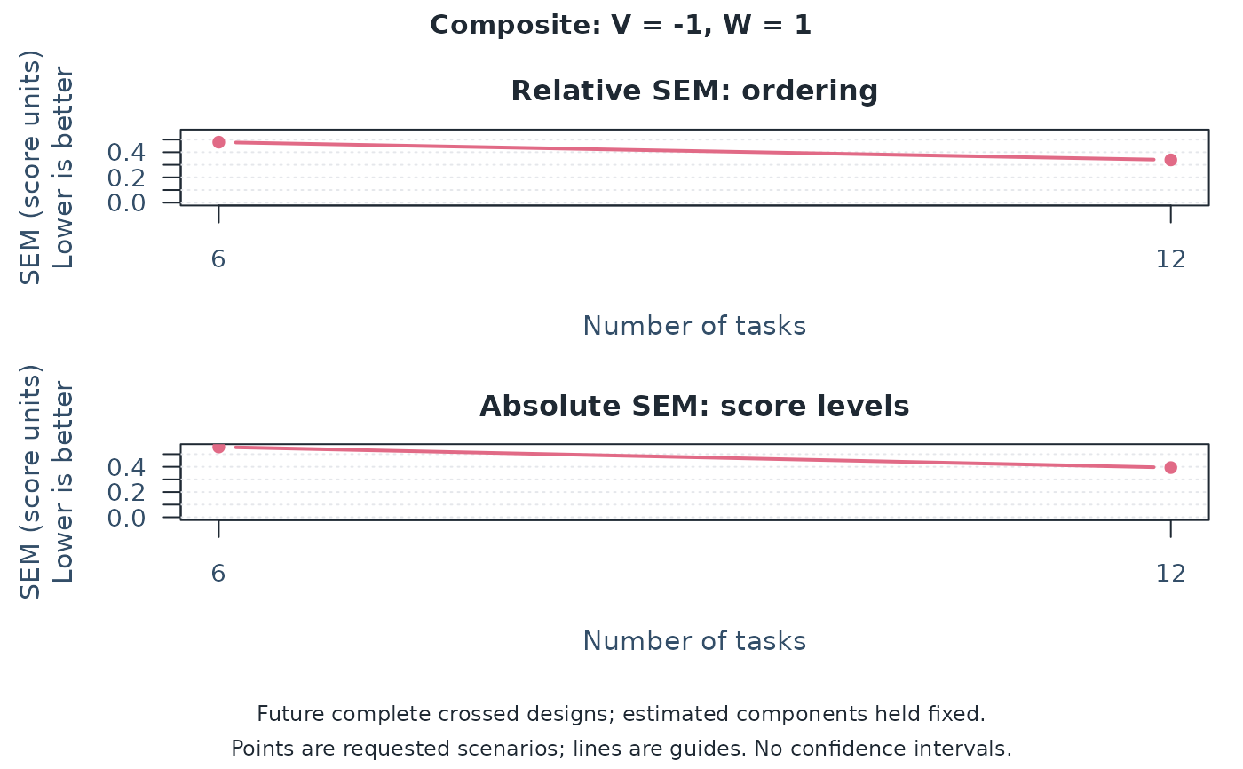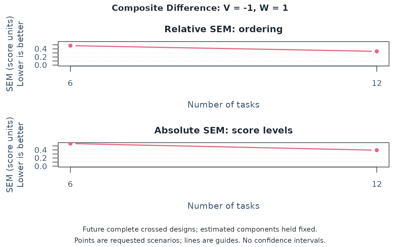plot(d, type = "sem") shows the SEMs. Plots select a sole composite by default, or the first score when there are no composites. 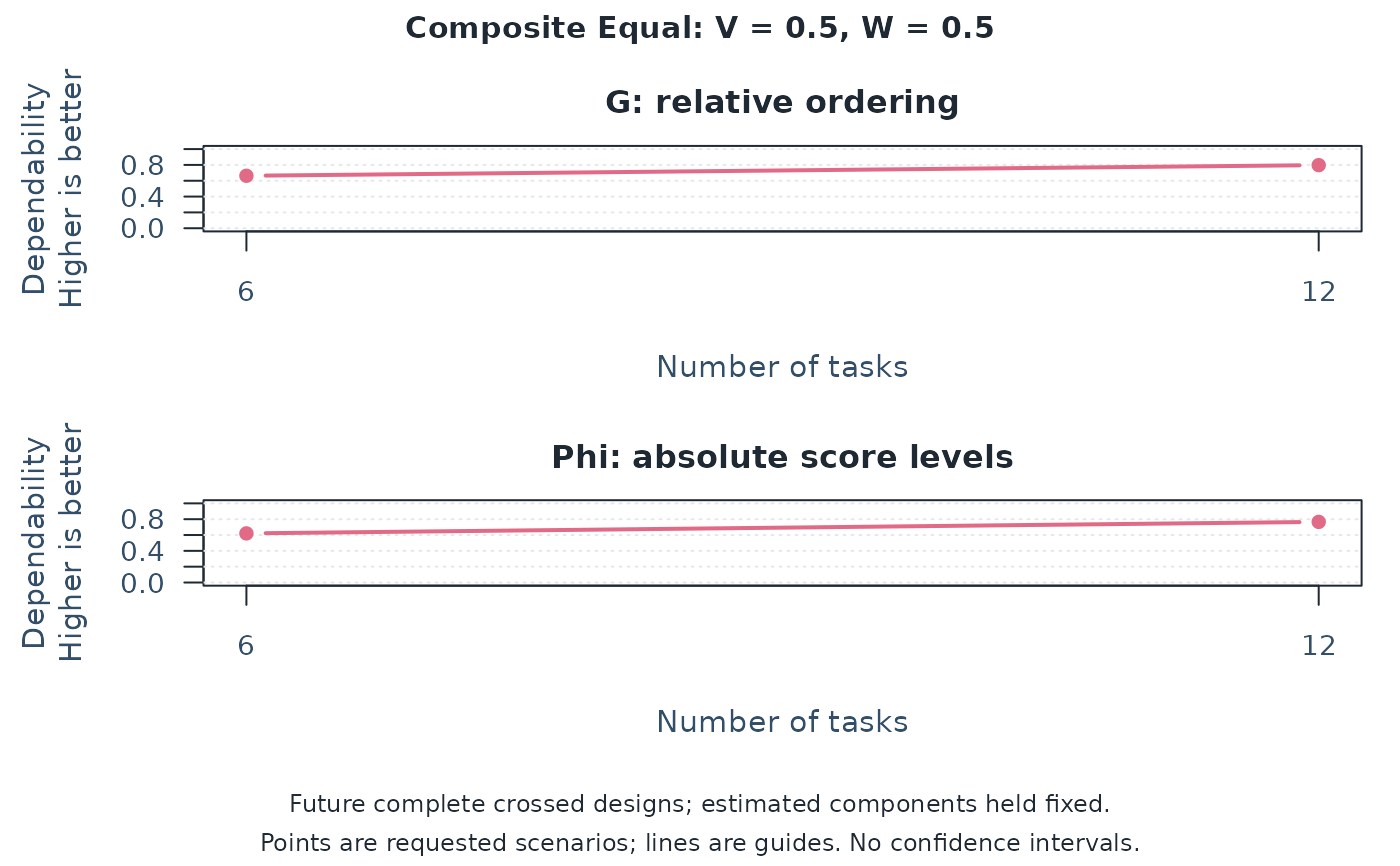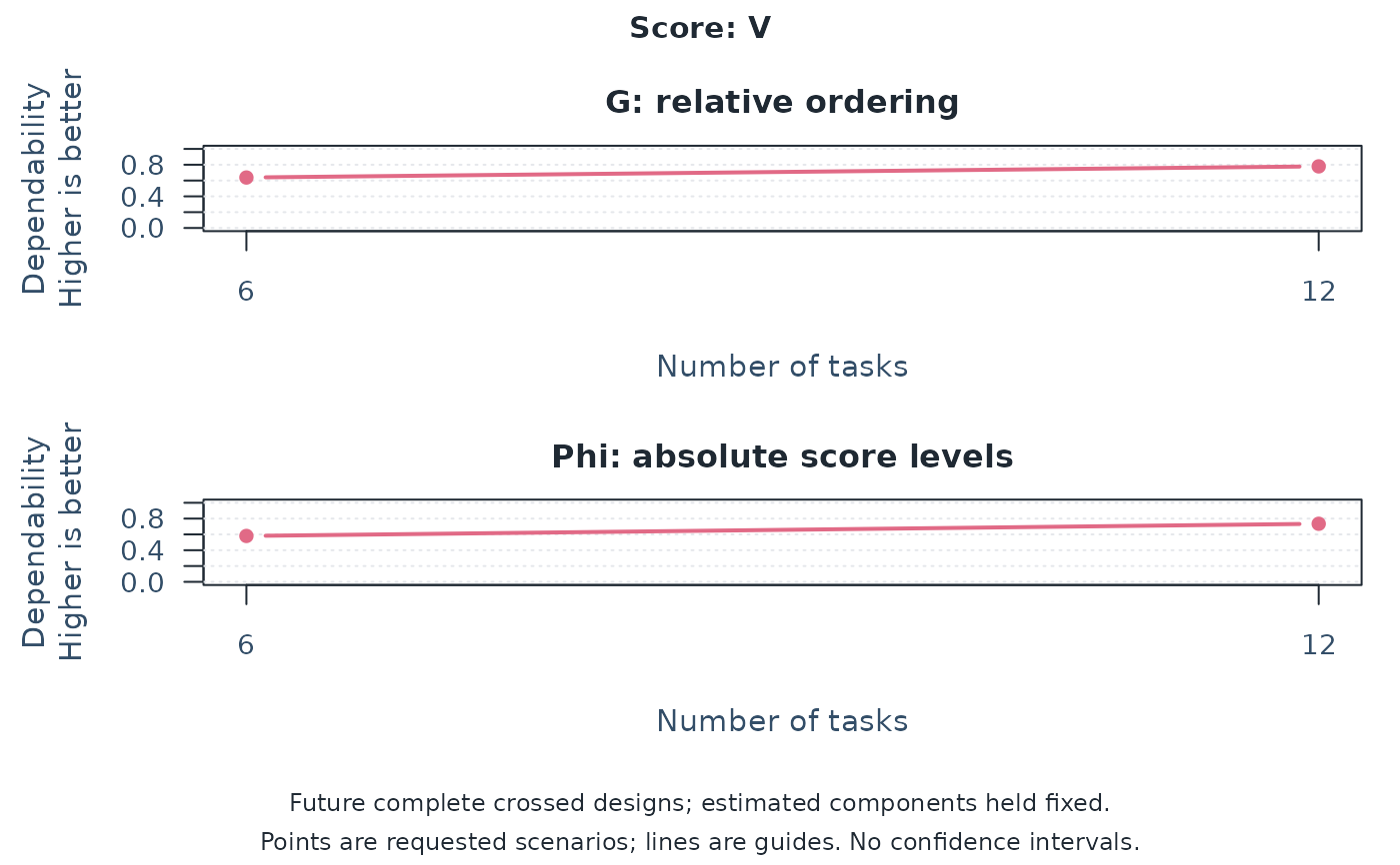With several composites, specify one with plot(d, composite = "Equal"); use plot(d, score = "V") to inspect an original score named V. The title always identifies the plotted score and any composite weights. Check GStatus, PhiStatus, RelativeSEMStatus, and AbsoluteSEMStatus: each explains the corresponding metric's availability. NA means unavailable, not zero dependability. ComponentPSD separately flags covariance components needing review. See plot.mfrm_multivariate_d_study() for interpreting curves and unavailable estimates.

Calculation and interpretation limits

For crossed covariance component matrices P, R, T, PR, PT, RT, and E, universe-score covariance is P. Relative-error covariance is PR/n_r + PT/n_t + E/(n_r*n_t). Absolute-error covariance adds R/n_r + T/n_t + RT/(n_r*n_t). The G-study number of persons does not divide individual-score universe variance. Holding a count constant does not turn its random facet into a fixed facet. Composite weights define linear score combinations. They do not implement score-dependent panel trimming or an entire competition scoring rule. For a Person-by-Task G-study, E combines Person-by-Task interaction and within-cell error: relative-error covariance is E/n_t, absolute-error covariance is (T + E)/n_t, and universe-score covariance remains P. The same formulas apply to a Person-by-Rater design or to facets selected by facets, with names replaced in the declared order. For a single facet F and its planned count n, relative error is E/n and absolute error is (F + E)/n. A D-study cannot introduce an absent facet. For fixed tasks represented by score columns in a Person-by-Rater model, vary only Raters. The task set remains fixed, and each planned rater scores all tasks. See "Fixed tasks as score components" in mfrm_multivariate_gstudy() for the target and allocation requirements.

For raters nested within tasks, use the five components P, T, R(T), PT, and E, where E includes the Person-by-Rater-within-Task interaction. With n_r raters per task and n_t tasks, relative error is PT/n_t + E/(n_r*n_t); absolute error adds T/n_t + R(T)/(n_r*n_t). Universe covariance remains P. Other nested facet labels follow the same rules. All persons receive the same tasks and their nested raters; two raters per task at six tasks means twelve distinct raters, not two raters each judging six tasks. Future unequal child counts, changes of nesting, and nested-design sampling intervals are not supported.

For incomplete source data, counts of distinct observed levels are not per-person replication counts. This function projects a future complete design; it does not estimate the reliability of the observed sparse roster, heterogeneous person-specific assignments, or averages of them.

Each score uses diagonal entries; a composite uses w' Sigma w for each of the three covariance matrices. Thus between-score covariance affects composite dependability. G = UniverseVariance / (UniverseVariance + RelativeErrorVariance) and Phi uses absolute error instead. SEMs are square roots of the corresponding error variances, in the units of the score or specified composite of mean scores. Multiplying all weights by a nonzero constant multiplies SEMs by its absolute value but leaves G/Phi unchanged. Weights express a substantive choice; this function neither chooses them nor identifies an optimal design. Interpret a difference only when subtraction is meaningful on the supplied score scales. Comparing several composites holds the estimated components and planned designs constant, but different weights may change the construct being assessed. A higher coefficient alone does not justify that change. Compare SEMs across composites only when their scales are comparable.

The same weights define the universe-score composite and its observed mean-score estimate (the equal WWTS/AWTS case in mGENOVA). Different target and estimation weights, profile reliability, and accuracy at a cut score are not provided. Unlike mGENOVA's default D-study procedure, negative variance estimates are not replaced with zero. mGENOVA replaces negative variance components with zero for the D-study unless its NEGATIVE option is selected (manual, pages 15 and 21). That rule concerns variances, not all negative covariances, and does not guarantee PSD component matrices. Do not transfer that option's meaning to jGENOVA: its NEGATIVE option controls printing of negative estimates. jGENOVA's D-study zeroes negative variances with either ALGORITHM or its default EMS convention; EMS also recalculates other components using the zero replacements. Matching a raw G-study estimate therefore need not give matching default D-studies. These conventions are not selectable estimation options in this function.

Raw covariance matrices and projected variances remain available. G requires nonnegative universe and relative-error variances and a positive sum; Phi uses absolute-error variance instead. Each SEM requires only its corresponding nonnegative error variance. A failed requirement makes only that metric NA. Zero universe variance yields a coefficient of zero when its error variance is positive; a zero total variance leaves the coefficient undefined. No estimates are clipped or replaced.

Status summarizes a row as "Available", "Partially available", or "Unavailable"; the four metric-specific status columns give the reasons. ComponentPSD is TRUE only when all G-study component matrices pass their numerical PSD check. A FALSE value flags components for review without suppressing otherwise calculable projections. Print and plot methods display a note for non-PSD components. Calculability does not validate the joint covariance model or establish precise estimation; inspect component_diagnostics before interpreting estimates. Raw estimates can yield Phi > G when projected absolute error is less than relative error. Under the stated model, the extra absolute-error contributions are nonnegative; such a reversal calls for review of the estimated components, not a conclusion that absolute decisions are more dependable. Passing the matrix checks does not establish model fit. Outputs are point projections conditional on the estimated components, without confidence intervals, missing-data correction, or MFRM latent inference.

References

Brennan, R. L. (2001). Generalizability theory. Springer. Chapters 9–11. Brennan, R. L. (2001). Manual for mGENOVA, Version 2.1. Iowa Testing Programs Occasional Papers, No. 50. Pages 16 and 20–22; Appendices E and F, pages 74–81. Crick, J. E., and Brennan, R. L. (2021). Manual for jGENOVA, Version 1.0. Pages 2-10–2-11, 3-5, and A-22–A-23.

Examples

# Published synthetic two-score data: the same six tasks for ten persons.
tasks <- read.csv(system.file("extdata", "mgenova-table12.csv", package = "mfrmr"))
g <- mfrm_multivariate_gstudy(tasks, c("V", "W"), rater = NULL)

# Question: would doubling tasks improve the dependability of W minus V?
d <- mfrm_multivariate_d_study(g, data.frame(Tasks = c(6, 12)),
  weights = c(V = -1, W = 1))
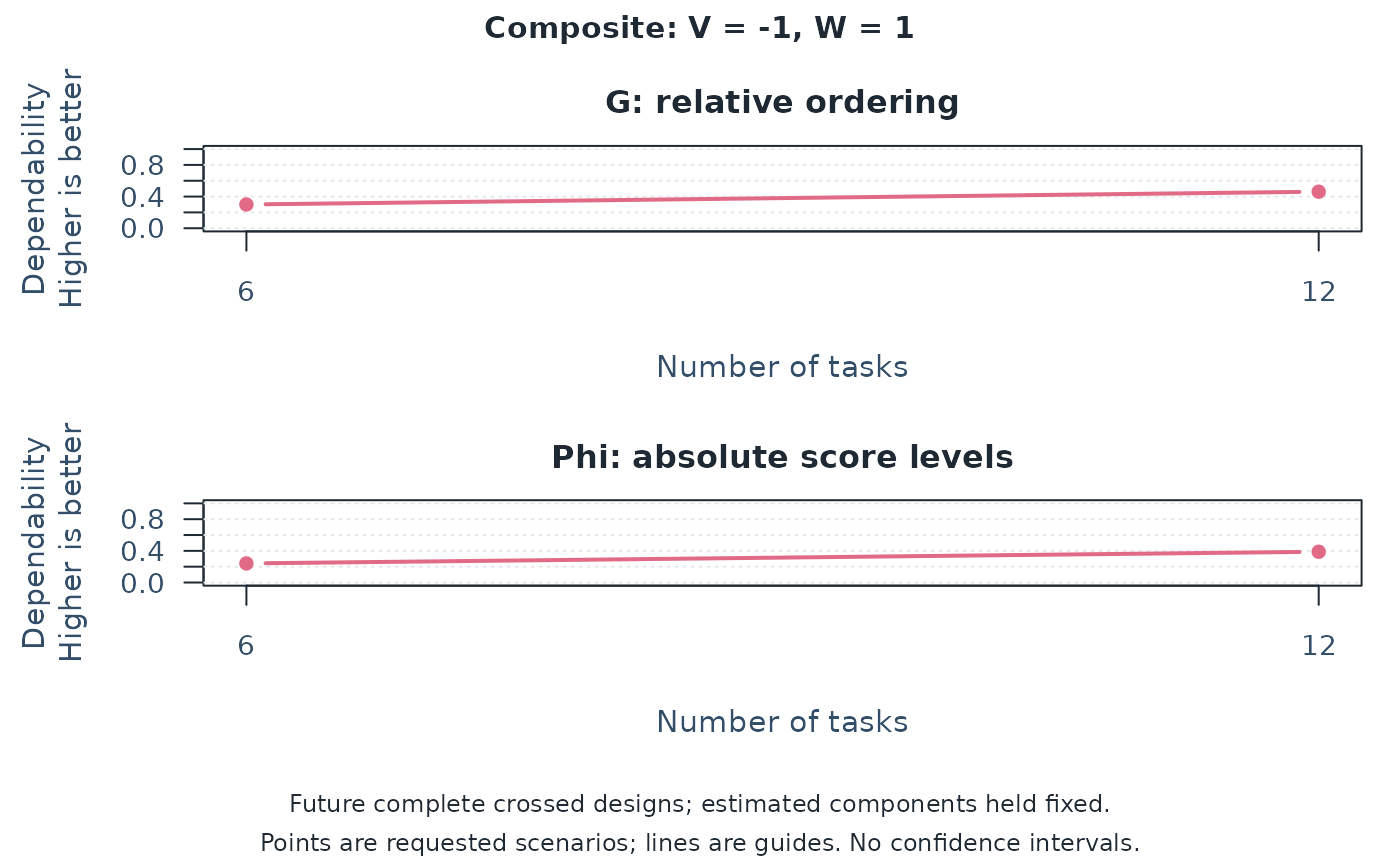
summary(d)
#>   Scenario Tasks      Kind     Score UniverseVariance RelativeErrorVariance
#> 1        1     6     Score         V       0.36814815             0.2087037
#> 2        1     6     Score         W       0.36888889             0.2561111
#> 3        1     6 Composite Composite       0.09851852             0.2298765
#> 4        2    12     Score         V       0.36814815             0.1043519
#> 5        2    12     Score         W       0.36888889             0.1280556
#> 6        2    12 Composite Composite       0.09851852             0.1149383
#>   AbsoluteErrorVariance         G       Phi RelativeSEM AbsoluteSEM    Status
#> 1             0.2661111 0.6382022 0.5804380   0.4568410   0.5158596 Available
#> 2             0.3094444 0.5902222 0.5438165   0.5060742   0.5562773 Available
#> 3             0.3100000 0.3000000 0.2411605   0.4794544   0.5567764 Available
#> 4             0.1330556 0.7791495 0.7345280   0.3230354   0.3647678 Available
#> 5             0.1547222 0.7423141 0.7045093   0.3578485   0.3933475 Available
#> 6             0.1550000 0.4615385 0.3886048   0.3390255   0.3937004 Available
#>     GStatus PhiStatus RelativeSEMStatus AbsoluteSEMStatus ComponentPSD
#> 1 Available Available         Available         Available         TRUE
#> 2 Available Available         Available         Available         TRUE
#> 3 Available Available         Available         Available         TRUE
#> 4 Available Available         Available         Available         TRUE
#> 5 Available Available         Available         Available         TRUE
#> 6 Available Available         Available         Available         TRUE
plot(d)

plot(d, type = "sem")

# G rises from 0.300 to 0.462, conditional on these estimated components.
# This is a planning projection, not evidence from twelve observed tasks.

# Without weights, report the original scores without creating a composite.
individual <- mfrm_multivariate_d_study(g, data.frame(Tasks = c(6, 12)))
plot(individual, score = "V")


# Compare weight choices on the same task-count scenarios.
weights <- cbind(Equal = c(V = 0.5, W = 0.5),
  W_focus = c(V = 0.2, W = 0.8), Difference = c(V = -1, W = 1))
alternatives <- mfrm_multivariate_d_study(g,
  data.frame(Tasks = c(6, 12)), weights = weights)
summary(alternatives) # Original scores plus all three named composites.
#>    Scenario Tasks      Kind      Score UniverseVariance RelativeErrorVariance
#> 1         1     6     Score          V       0.36814815            0.20870370
#> 2         1     6     Score          W       0.36888889            0.25611111
#> 3         1     6 Composite      Equal       0.34388889            0.17493827
#> 4         1     6 Composite    W_focus       0.35297778            0.20984938
#> 5         1     6 Composite Difference       0.09851852            0.22987654
#> 6         2    12     Score          V       0.36814815            0.10435185
#> 7         2    12     Score          W       0.36888889            0.12805556
#> 8         2    12 Composite      Equal       0.34388889            0.08746914
#> 9         2    12 Composite    W_focus       0.35297778            0.10492469
#> 10        2    12 Composite Difference       0.09851852            0.11493827
#>    AbsoluteErrorVariance         G       Phi RelativeSEM AbsoluteSEM    Status
#> 1              0.2661111 0.6382022 0.5804380   0.4568410   0.5158596 Available
#> 2              0.3094444 0.5902222 0.5438165   0.5060742   0.5562773 Available
#> 3              0.2102778 0.6628198 0.6205514   0.4182562   0.4585605 Available
#> 4              0.2511778 0.6271513 0.5842498   0.4580932   0.5011764 Available
#> 5              0.3100000 0.3000000 0.2411605   0.4794544   0.5567764 Available
#> 6              0.1330556 0.7791495 0.7345280   0.3230354   0.3647678 Available
#> 7              0.1547222 0.7423141 0.7045093   0.3578485   0.3933475 Available
#> 8              0.1051389 0.7972238 0.7658521   0.2957518   0.3242513 Available
#> 9              0.1255889 0.7708580 0.7375728   0.3239208   0.3543852 Available
#> 10             0.1550000 0.4615385 0.3886048   0.3390255   0.3937004 Available
#>      GStatus PhiStatus RelativeSEMStatus AbsoluteSEMStatus ComponentPSD
#> 1  Available Available         Available         Available         TRUE
#> 2  Available Available         Available         Available         TRUE
#> 3  Available Available         Available         Available         TRUE
#> 4  Available Available         Available         Available         TRUE
#> 5  Available Available         Available         Available         TRUE
#> 6  Available Available         Available         Available         TRUE
#> 7  Available Available         Available         Available         TRUE
#> 8  Available Available         Available         Available         TRUE
#> 9  Available Available         Available         Available         TRUE
#> 10 Available Available         Available         Available         TRUE
plot(alternatives, composite = "Equal")

plot(alternatives, composite = "Difference", type = "sem")

# Choose weights for the intended interpretation, not solely for higher G.