Portable calibration and fresh-session scoring • mfrmr

This workflow creates a portable calibration from an eligible fitted model, validates and freezes it, saves it, and then scores new Persons without the source fit or training responses. The scoring phase uses only the saved artifact and the new response rows.

The portable workflow is deliberately narrower than fitted-object scoring. It supports one observed score scale and one latent dimension. RSM and PCM MML use the fixed standard-normal calibration basis (file format 1). In the development version, GPCM MML also supports an estimated intercept-only normal population (file format 2), one positive slope family and shared or separate slope/step owners. GPCM requires unit weights and no anchors or interactions. RSM/PCM JML also supports post-hoc EAP from a portable artifact (file format 3), with a finite identified source, unit weights and no anchors or interactions. Shared-owner GPCM JML uses file format 4 after passing its conditional joint-likelihood and curvature checks. Experimental corrected shared-owner GPCM JML uses file format 5 with fresh adjusted-equation checks, an explicit correction order and a separate post-hoc normal reference prior. Its finite EAPs are not corrected Person maxima; calibration uncertainty and residual bias are not included in posterior intervals. See the corrected-JML example in vignette("mfrmr-gpcm-scope", package = "mfrmr"). Estimated-population RSM/PCM and latent regression remain fitted-object-only routes.

Experimental two-family GPCM MML uses file format 6 with the same public lifecycle below. It retains two ordered slope owners, second-owner steps, the original category coding and fixed N(0,1) prior. The first owner’s locations and log slopes are centered; the second owner’s locations and slopes remain free. Source identity/convergence and finer-integration checks must pass before extraction; review-only sources cannot be frozen. Each scoring batch must pass its own EAP/SD integration checks. Both fixed-grid EM and adaptive direct MML retain their scoring integration method.

The artifact contains no training responses or Person estimates. Known facet levels may form new combinations, flagged by row_dispositions$ObservedContext; this is a model-based extension, not empirical validation of those combinations. Unit weights are required, with no prior override or repeated-event extension. Facet names must not collide with the reserved scoring/disposition columns listed in ?mfrm_calibration_workflow. Validation and freezing do not qualify sampling coverage, global identification or population transport, and intervals exclude calibration uncertainty. Older readers refuse format 6; formats 1–5 retain their interpretation. See the two-family example in the GPCM scope vignette.

For a JML source, EAP holds the calibration fixed and adds a standard-normal reference prior by default, or uses an explicit scoring_prior. JML did not estimate that distribution. This is not ML/WLE scoring or a replay of the original joint Person estimates. A full fit saved with saveRDS() and a portable calibration are different objects; only the latter omits training responses and Person estimates. See the GPCM scope vignette for the MML/JML feature comparison.

For RSM/PCM MML, supported direct and group facet anchors and two-way facet interactions are retained in the calibration. New responses must use its recorded non-Person facet levels. Preserving an interaction for scoring does not establish its statistical significance or the model’s suitability for another population.

library(mfrmr)

mfrm_calibration_capabilities()[, c(
  "Model", "Estimator", "ScoringBasis", "PortableCalibration"
)]
#>                 Model     Estimator                              ScoringBasis
#> 1                 RSM           MML                     fixed standard normal
#> 2                 PCM           MML                     fixed standard normal
#> 3             RSM/PCM           MML estimated population or latent regression
#> 4                GPCM           MML    frozen estimated intercept-only normal
#> 5             RSM/PCM           JML        post-hoc standard normal reference
#> 6                GPCM           JML        post-hoc standard normal reference
#> 7                GPCM Corrected JML        post-hoc standard normal reference
#> 8 GPCM (two families)           MML                     fixed standard normal
#>   PortableCalibration
#> 1           available
#> 2           available
#> 3         unavailable
#> 4           available
#> 5           available
#> 6           available
#> 7           available
#> 8           available

Calibration session

The bundled example_core data are synthetic. This example uses 18 Persons to keep vignette runtime modest; a substantive analysis should use its planned sample and design rather than copying that count.

synthetic <- load_mfrmr_data("example_core")
person_ids <- unique(as.character(synthetic$Person))
training_ids <- person_ids[seq_len(18L)]
training <- synthetic[
  as.character(synthetic$Person) %in% training_ids,
  ,
  drop = FALSE
]

fit <- suppressWarnings(fit_mfrm(
  training,
  person = "Person",
  facets = c("Rater", "Criterion"),
  score = "Score",
  model = "RSM",
  method = "MML",
  quad_points = 5,
  maxit = 20
))

quadrature_review <- suppressWarnings(mml_quadrature_sensitivity(
  fit,
  training,
  quad_points = c(5, 7),
  theta_points = 41
))
summary(quadrature_review)
#> RSM-MML quadrature sensitivity summary
#>  ReferenceNodes ComparedGrids AllEstimationConverged AllHessiansFullRank
#>               5             2                   TRUE                TRUE
#>  MaxNLLAbsChangePerPerson MaxMeasurementParameterAbsChange MaxSlopeAbsChange
#>                   0.09056                          0.06055                NA
#>  MaxPopulationSDAbsChange MaxProbabilityAbsChange MaxEAPAbsChange
#>                         0                 0.01598         0.47415
#>  MaxPosteriorSDAbsChange
#>                  0.29125
#> 
#> Grid comparisons
#>  Model ReferenceNodes Nodes IsReference NLLChangePerPerson
#>    RSM              5     5        TRUE            0.00000
#>    RSM              5     7       FALSE           -0.09056
#>  NLLAbsChangePerPerson MeasurementParameterMaxAbsChange SlopeMaxAbsChange
#>                0.00000                          0.00000                NA
#>                0.09056                          0.06055                NA
#>  RawSlopeSEMaxAbsChange SlopeIntervalMaxAbsChange
#>                      NA                        NA
#>                      NA                        NA
#>  SlopeIntervalEligibilityChanged PopulationSDAbsChange
#>                               NA                     0
#>                               NA                     0
#>  RawPopulationSDSEAbsChange ProbabilityMaxAbsChange EAPMaxAbsChange
#>                          NA                 0.00000         0.00000
#>                          NA                 0.01598         0.47415
#>  PosteriorSDMaxAbsChange
#>                  0.00000
#>                  0.29125
#> No automatic stability classification or readiness change is applied.
fit <- quadrature_review$fits$q7

draft <- extract_mfrm_calibration(
  fit,
  calibration_id = "portable-rsm-example",
  source_fit_id = "synthetic-rsm-fit",
  scoring_quad_points = 31,
  quadrature_review = quadrature_review
)
review_mfrm_calibration(draft)
#> [1] Code      FieldPath Detail    Severity 
#> <0 rows> (or 0-length row.names)

validated <- validate_mfrm_calibration(draft)
frozen <- freeze_mfrm_calibration(validated)
frozen
#> <mfrm_calibration>
#>   State: frozen
#>   Model: RSM / MML
#>   Scoring prior: standard normal (mean 0, SD 1)
#>   Facets: 2; coordinates: 11; anchors: 0
#>   Validation refusals: 0

artifact_file <- tempfile(fileext = ".rds")
save_mfrm_calibration(frozen, artifact_file)

The fit-time quadrature and the scoring-time quadrature are distinct. The two small fit grids above keep this example quick; they are not recommendations for substantive work. Inspect the continuous movement on grids chosen for the application and extend them when needed. Public extraction accepts the exact highest-grid fit in that review but does not decide whether its movement is small enough. The artifact separately records the 31-point grid used for later posterior scoring, and the response-linked review should be archived outside the portable artifact when it is needed for an audit trail.

Fresh scoring session

In operational use, start a new R process and supply only the artifact path and new response rows. The following chunk removes the fit, draft, validation object, and training data before loading the artifact, so none can influence the score.

new_rows <- synthetic[
  as.character(synthetic$Person) %in% person_ids[19:20],
  c("Person", "Rater", "Criterion", "Score"),
  drop = FALSE
]
new_ids <- stats::setNames(
  c("NEW_PERSON_1", "NEW_PERSON_2"), person_ids[19:20]
)
new_rows$Person <- unname(new_ids[as.character(new_rows$Person)])
rownames(new_rows) <- NULL

# Create one explicit review case for the tutorial figure. In operational
# scoring, never alter observed responses to manufacture a disposition.
new_rows$Score[new_rows$Person == "NEW_PERSON_2"] <- max(training$Score)

rm(fit, quadrature_review, draft, validated, frozen, training, synthetic)
invisible(gc())

calibration <- load_mfrm_calibration(artifact_file)
scores <- score_mfrm_calibration(
  calibration, new_rows, adaptive_quad_points = c(31, 61)
)
summary(scores)
#> mfrmr Portable Calibration Score Summary
#> 
#> Fixed-parameter integration review (adaptive minus fixed)
#>  FixedNodes AdaptiveNodes Persons Unavailable MaxAbsLogMarginalChange
#>          31            31       2           0             0.002445619
#>          31            61       2           0             0.002445619
#>  MaxAbsEAPChange MaxAbsSDChange
#>      0.002926627     0.00356594
#>      0.002926627     0.00356594
#>   Calibration: portable-rsm-example
#>   Model / estimator: RSM / MML
#>   Persons: 2 scored (1 requiring review); 0 not scored
#> 
#> Posterior estimates (2 of 2)
#>   NEW_PERSON_1: estimate 0.959, SD 0.328, interval [0.331, 1.605], scored
#>   NEW_PERSON_2: estimate 3.135, SD 0.529, interval [2.171, 4.244], review
#>   required
#> 
#> Persons requiring review or not scored (1 of 1)
#>   NEW_PERSON_2: review required; reasons: all responses at the maximum score
#> 
#> Response-row disposition
#>   32 input; 32 scored; 0 omitted; 0 refused; missing-response policy: error
#> 
#> Interval interpretation
#>   95% intervals: continuous posterior quantiles.
#>   Posterior SDs and intervals are conditional on the frozen point calibration
#>   and exclude calibration-parameter uncertainty.

plot(
  scores,
  type = "interval",
  preset = "publication"
)

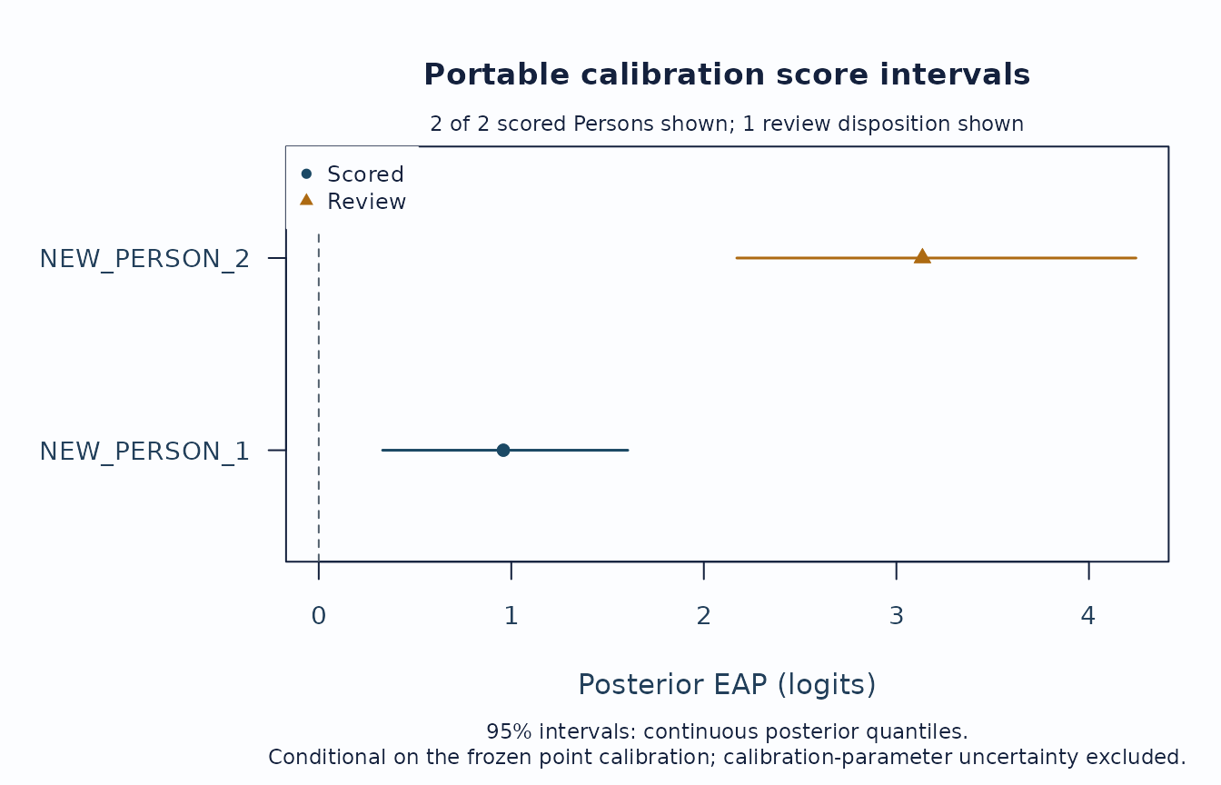
Posterior EAP intervals for two newly scored Persons. A blue circle marks a conditionally ready score, an orange triangle marks a score requiring review, and a dashed vertical line marks the zero-logit scale origin.


unlink(artifact_file)

The base and optional ggplot2 renderers distinguish scored and review states by shape as well as colour. The complete score and review tables remain in the summary object even though its console printout shows only a compact preview.

The interval figure is the first score-batch review. Orange triangles identify Persons whose Disposition is scored_review; inspect their ReasonCodes before using the estimate. A Person with no valid response has no score coordinate and therefore appears in summary(scores)$review and in the draw-free plot payload’s unplotted_dispositions, not as an artificial point.

Two focused follow-up views use the same score object without consulting the source fit:

# Valid response rows versus posterior SD.
plot(scores, type = "precision", preset = "publication")

# Posterior mass on the outer quadrature nodes versus the recorded threshold.
edge_review <- plot(scores, type = "edge_mass", draw = FALSE)
edge_review$data$selection_summary
edge_review$data$unplotted_dispositions

These displays review a returned score batch. They do not establish source-fit quality, reliability, calibration transport, or validity. Every interval and posterior SD remains conditional on the frozen point calibration and excludes calibration-parameter uncertainty.

A small edge mass does not guarantee accurate integration: a narrow posterior can fall between nodes near the middle of the grid. The optional adaptive_quad_points above adds a separate numerical comparison, placing nodes around each scored Person’s posterior mode and scaling their spacing to its local width. It holds the calibration parameters and prior fixed.

summary(scores)$quadrature_overview
#>   FixedNodes AdaptiveNodes Persons Unavailable MaxAbsLogMarginalChange
#> 1         31            31       2           0             0.002445619
#> 2         31            61       2           0             0.002445619
#>   MaxAbsEAPChange MaxAbsSDChange
#> 1     0.002926627     0.00356594
#> 2     0.002926627     0.00356594
# Keep full precision when inspecting individual differences.
head(scores$quadrature_review[c(
  "Person", "AdaptiveNodes", "EAPChange", "PosteriorSDChange",
  "AdaptiveEAPChangeFromPrevious", "AdaptiveSDChangeFromPrevious", "Status"
)])
#>         Person AdaptiveNodes     EAPChange PosteriorSDChange
#> 1 NEW_PERSON_1            31 -2.926627e-03      -3.56594e-03
#> 2 NEW_PERSON_1            61 -2.926627e-03      -3.56594e-03
#> 3 NEW_PERSON_2            31 -1.563277e-05       1.99646e-05
#> 4 NEW_PERSON_2            61 -1.563277e-05       1.99646e-05
#>   AdaptiveEAPChangeFromPrevious AdaptiveSDChangeFromPrevious   Status
#> 1                            NA                           NA computed
#> 2                 -1.332268e-15                -2.220446e-16 computed
#> 3                            NA                           NA computed
#> 4                  7.105427e-15                 1.005862e-13 computed

Check fixed-versus-adaptive differences and changes between adaptive orders, including log-marginal likelihood contributions in the full table. Observation weights, when supplied, enter the likelihood as in the original scoring call. The first adaptive order has no previous order, so its change columns are NA. A computed status means the calculation finished; it does not certify accuracy. An unavailable row retains the reason in Detail. Persons with no scored responses remain in the ordinary disposition review and have no numerical integration row. Archive the full table with the score batch when reporting numerical checks. The comparison does not replace returned scores, intervals, or the artifact’s stored grid, and it does not change readiness. Use the same option in predict_mfrm_units() or mml_quadrature_sensitivity() to review a fitted object; the latter also retains its separate comparison of refitted models.

To use adapted grids during fitting and subsequent scoring, set mml_integration = "adaptive" in the fit_mfrm() call above. The direct MML engine then updates the grids while estimating parameters. The refit review retains this mode, and the frozen artifact records scoring_algorithm = "adaptive_quadrature_eap_v2". Its stored nodes and weights define the base Hermite rule; scoring places that rule around each new Person’s posterior. A small edge mass on an adapted grid is still not an accuracy certificate. Keep the order comparison and report the integration mode. Ordinary fitting defaults to mml_integration = "fixed", and existing fixed-grid artifacts retain their scoring algorithm.

New v2 scoring uses continuous equal-tail posterior intervals: a 95% interval leaves 2.5% of the continuous posterior below each lower endpoint and above each upper endpoint. EAP and SD still use the stored quadrature rule. Older v1 artifacts retain their discrete grid endpoints for reproducibility and carry a note that their continuous posterior mass may differ from the requested level. A frozen point calibration’s intervals exclude calibration-parameter uncertainty; they do not guarantee 95% coverage at every fixed true ability.

Printed results and interval plots state the requested level and identify saved grid-based intervals. Both scores$estimates and summary(scores)$estimates retain ScoringAlgorithm and IntervalLevel for CSV export, alongside the calibration and uncertainty basis. IntervalLevel is the requested posterior probability, not measured frequentist coverage, and is not rounded by summary(). For older saved score results, re-running summary() recovers these fields from the result’s stored settings without recomputing scores.

The scoring prior is also an assumption about the target population. For example, a new population with a wider ability distribution than the recorded standard normal prior can have less than 95% of its true abilities inside these intervals, even when the numerical integration is accurate. Increasing the quadrature order checks approximation under the same prior; it does not establish that this prior fits the new population. Report the scoring prior and explain its relevance to the population receiving scores, alongside the calibration and integration settings.

An intercept-only normal population fitted to training data can adjust the scoring mean and variance, but it does not learn a skewed population shape. Its score intervals still condition on the estimated calibration and population parameters and exclude uncertainty from estimating them. Training and scoring populations also need not match. Conditional fitted-object scoring can pass fresh local likelihood, gradient, information and integration checks without requiring a review override. GPCM fits passing these checks can also be exported within the scope above. This does not certify a global maximum or resolve unevaluated boundary/identification audits. Those original states remain in the artifact; loading checks the stored records, not the omitted training data.

For example, a calibration may come from last year’s cohort while this year’s cohort has a different ability distribution. With an intercept-only population model, scoring the new response batch retains the fitted mean and variance; it does not estimate a new batch population. Source readiness alone therefore does not establish that the prior represents this year’s people. Identify the training and scoring cohorts in the report, explain why the scoring prior can be applied to the new cohort, and examine sensitivity when that assumption is uncertain. A larger training sample can estimate last year’s population more precisely without resolving a difference between the two populations.

Reuse a GPCM calibration for a later cohort

Suppose a team uses the same rubric and known raters to score next year’s performances. The calibration describes the relationships between categories, facet effects and ability. The later session applies those fixed relationships; it does not recalibrate raters or estimate the new cohort’s distribution.

Use the full planned calibration sample, not the 18-person RSM illustration above. Each row in calibration_responses represents an assigned rating, with columns Person, Rater, Criterion and Score. This model gives criteria their own discriminations and raters their own category thresholds. For rater-owned discriminations instead, set slope_facet = "Rater". The 0–2 category ladder is an example: specify the actual rubric’s score range.

library(mfrmr)
calibration_responses <- read.csv(
  "calibration-responses.csv", colClasses = "character", na.strings = "",
  check.names = FALSE, fileEncoding = "UTF-8-BOM"
)
gpcm_fit <- fit_mfrm(
  calibration_responses,
  person = "Person", facets = c("Rater", "Criterion"), score = "Score",
  model = "GPCM", method = "MML",
  step_facet = "Rater", slope_facet = "Criterion",
  rating_min = 0, rating_max = 2, category_policy = "preserve",
  mml_integration = "adaptive", quad_points = 31,
  maxit = 400, reltol = 1e-10
)
summary(gpcm_fit, profile = "fit", detail = "brief")

These settings are a starting configuration, not a convergence or sample-size guarantee. Inspect the fit and its warnings. Extraction checks the calibration before it can be frozen; increasing only the later scoring grid cannot repair a failed calibration check. A profile interval for a discrimination is a separate experimental option, not a required step in scoring or an interval for a new person’s ability. Once gpcm_fit has passed calibration review:

draft <- extract_mfrm_calibration(
  gpcm_fit, calibration_id = "rubric-calibration",
  source_fit_id = "training-cohort", scoring_quad_points = 141
)
review_mfrm_calibration(draft)
calibration <- freeze_mfrm_calibration(validate_mfrm_calibration(draft))
save_mfrm_calibration(calibration, "gpcm-calibration.rds")

In a new R session, read that artifact and the later cohort’s responses:

library(mfrmr)
# A later session needs only this file and the new response rows.
calibration <- load_mfrm_calibration("gpcm-calibration.rds")
new_responses <- read.csv(
  "new-responses.csv", colClasses = "character", na.strings = "",
  check.names = FALSE, fileEncoding = "UTF-8-BOM"
)
scores <- score_mfrm_calibration(
  calibration, new_responses, missing_response = "omit"
)
score_review <- summary(scores)
score_review
score_review$review
score_review$settings$score_integration_review
plot(scores, type = "interval", preset = "publication", top_n = Inf)

# Keep full-precision scores and every Person's disposition, including those
# without scores. The complete object supports later review and plotting.
write.csv(scores$estimates, "person-scores.csv", row.names = FALSE, na = "")
write.csv(scores$person_dispositions, "person-review.csv", row.names = FALSE, na = "")
saveRDS(scores, "scored-cohort.rds")

The omission policy applies to assigned ratings whose score is missing. It does not impute scores or repair informative missingness. Leave unassigned rating combinations absent rather than manufacturing observations. A person with only missing assigned scores remains not_scored in the review table, with no plotted point. A person entirely absent from the input is not invented by the scorer. Keep the review file with the score file so unavailable results do not disappear. Identifiers 001, 1 and the literal NA stay distinct with the character-column import above.

top_n = Inf displays every available score; the default is at most 40, with review cases prioritized. For a large cohort use a legible subset and retain the complete tables. After readRDS("scored-cohort.rds"), summary(), plot() and as_ggplot() reuse saved results without fitting or scoring again.

The summary distinguishes the actual reported-score integration check from the additional fixed-versus-adaptive grid comparison. For an adaptive scorer, a difference from an unused fixed grid does not contradict passing agreement of the reported EAP/SD with higher-order adaptive references.

retained <- scores$settings$retained_prior_identity

# Sensitivity analysis on the same calibration scale, not a new population fit.
alternative <- score_mfrm_calibration(
  calibration, new_responses, missing_response = "omit",
  scoring_prior = list(mean = retained$mean + 0.5, sd = retained$sd * 1.25)
)
summary(alternative)

The shift of 0.5 logits and 25% wider SD illustrate a declared assumption; they are not recommended prior values. Compare the same people, retain both priors and justify substantive scenarios. These posterior score intervals condition on the calibration and prior. They differ from confidence intervals for estimated slopes or facet parameters.

For the training-model report, use mfrm_results(gpcm_fit) and mfrm_report() in the calibration session. For the later score batch, use the dedicated summary, plots, CSV tables and saved score object above. mfrm_report() does not accept portable score batches; a report of the training fit does not become a report of the new cohort.

There are two distinct checks. Extraction evaluates the estimated calibration using the training fit. Scoring checks the new response patterns under the actual prior. A calibration that passes the first check can still require a finer scoring grid for extreme new patterns. If scoring stops with SCORING_INTEGRATION_FAILED, extract again with more scoring_quad_points and repeat validation and freezing; 141 is an example, not a universal adequate order. There is no review override for failed portable numerical checks. Passing them does not remove endpoint or sparse-response review labels.

The default retains the estimated normal mean and SD from calibration. scoring_prior supplies an assumption for sensitivity analysis; it does not estimate the later cohort’s distribution or change the saved calibration. Both original and actual prior values remain in score tables, summaries and plot data. Intervals condition on these fixed values and exclude uncertainty from estimating the calibration and its population. The same prior option is available for current RSM/PCM artifacts; older artifacts using grid-endpoint intervals require re-extraction first.

For a separate scoring script, the essential code is:

library(mfrmr)

calibration <- load_mfrm_calibration("reviewed-calibration.rds")
new_rows <- read.csv(
  "new-responses.csv",
  colClasses = "character",
  na.strings = "",
  check.names = FALSE,
  fileEncoding = "UTF-8-BOM"
)
scores <- score_mfrm_calibration(calibration, new_rows)
print(scores)
plot(scores, type = "interval", preset = "publication")
write.csv(scores$estimates, "person-scores.csv", row.names = FALSE)

Read identifiers as text: 001 and 1 can identify different Persons, and NA can be a literal identifier. The example treats empty cells as missing; if your response file uses another missing-score token, convert it only in the score column before scoring. Do not let automatic CSV type conversion merge people or change the frozen facet labels. Numeric score strings are validated against the frozen score map by the scorer.

Keep scores with saveRDS() when the full review and numerical settings are needed. The CSV above preserves per-score identities and uncertainty labels, but does not contain the complete row review or optional integration review. When reading that CSV back, also preserve identifier columns as text.

Unknown facet levels, unknown score values, invalid weights, ambiguous duplicates, and malformed artifacts fail closed. Missing responses require an explicit missing_response = "omit" policy.

If scoring stops or asks for review

An input error stops the scoring call. A returned scored_review result has an estimate that needs review; not_scored means no estimate is available. Inspect summary(scores)$review, including Persons absent from the interval plot. The printed review translates the reason codes into descriptions.

What you see	What to check or change
An unseen rater, task, or other facet level	Check spelling and preserve IDs as text. A genuinely new level has no parameter in this calibration: return to calibration with an appropriate linking design. Do not rename it as an existing level or edit the frozen artifact.
A score outside the frozen map	Check the original rubric and missing-score codes. Correct an entry error or explicitly recode a documented missing marker. A changed rubric requires calibration review; widening a score range cannot update the saved map.
Missing scores or IDs	Correct unintended missing values. Explicit omission applies to missing scores, not missing Person or facet IDs, and does not correct selective nonresponse. Review omitted counts after rescoring.
Duplicate response cells	Check whether rows are accidental copies or distinct rating events. Correct copies; use the documented `event_id` argument only for genuine distinct events under the intended model. New event IDs do not model dependence between repeated performances.
A missing, nonfinite, or nonpositive weight on a scored row	Check the weight column and its intended meaning. Correct erroneous values; do not replace them with arbitrary constants just to obtain scores.
A malformed or incompatible artifact	Restore the original file and use a compatible package version. If it must be recreated, return to the source fit and the documented extraction/review workflow. Do not edit schema or validation fields to bypass the refusal.
Review because responses are very few, omitted, or all at one endpoint	Check the original ratings and valid/omitted counts. Interpret precision and dependence on the prior before using the estimate; further ratings may be needed. These flags do not by themselves diagnose an invalid Person or justify changing responses.
Review because posterior mass is near integration limits	Examine the numerical comparisons described above. Increasing optimizer iterations cannot alter a frozen calibration. If scoring settings need revision, return to the calibration workflow and retain a new artifact and its review.
No valid responses (`not_scored`)	Correct missing-score coding if erroneous, or obtain valid ratings. Retain the unavailable result; do not substitute a zero-logit score.

A completed numerical comparison does not automatically clear these review states. Record the reason, the action taken, and the calibration used with the score batch.

Every returned estimate is a posterior EAP conditional on the recorded fixed point calibration and prior; its uncertainty interval excludes calibration-parameter uncertainty. Validate the intended score use, population transport, and decision consequences outside this numerical workflow.

When the calibration was estimated with JML

Suppose raters have already scored one cohort, and you want to score a later cohort using their existing severity estimates. RSM/PCM JML can now use the same extract/validate/freeze/save/load/score functions. Extraction checks a current, finite, identified source and freshly evaluates its joint likelihood and gradient. It does not use mml_quadrature_sensitivity(), because JML calibration does not integrate over a population distribution. An unresolved source is refused, not automatically switched to MML or made acceptable by a scoring prior.

The following PCM example uses 14 synthetic learners for a small illustration, not as a sample-size recommendation. Its 141-node scoring grid is also an example, not a generally sufficient setting. Each new batch receives integration checks; if those fail, inspect the error and increase scoring_quad_points when extracting.

library(mfrmr)
jml_data <- load_mfrmr_data("example_core")
jml_data <- jml_data[jml_data$Person %in% unique(jml_data$Person)[1:14], ]
jml_fit <- fit_mfrm(jml_data, "Person", c("Rater", "Criterion"), "Score",
  model = "PCM", method = "JML", step_facet = "Criterion",
  maxit = 500, reltol = 1e-10)
jml_draft <- extract_mfrm_calibration(jml_fit, scoring_quad_points = 141)
jml_calibration <- freeze_mfrm_calibration(validate_mfrm_calibration(jml_draft))
save_mfrm_calibration(jml_calibration, "jml-calibration.rds")

# In a new session, supply your later cohort's ratings instead of these example rows.
jml_new <- jml_data[jml_data$Person == unique(jml_data$Person)[1], ]
jml_new$Person <- "NEXT01"
jml_saved <- load_mfrm_calibration("jml-calibration.rds")
jml_scores <- score_mfrm_calibration(jml_saved, jml_new)
summary(jml_scores)
plot(jml_scores, main = "New-cohort EAP scores")

jml_alternative <- score_mfrm_calibration(jml_saved, jml_new,
  scoring_prior = list(mean = 0.25, sd = 1.2))
jml_scores$estimates[, c("Person", "Estimate", "SD", "PriorMean", "PriorSD")]
jml_alternative$estimates[, c("Person", "Estimate", "SD", "PriorMean", "PriorSD")]

For a ggplot without headings or a caption, use as_ggplot(jml_scores) + ggplot2::labs(title = NULL, subtitle = NULL, caption = NULL). Keep the interval interpretation in the surrounding report if you remove it from the figure.

The default N(0,1) prior is a reference assumption on the JML calibration scale, not an estimate of either cohort’s distribution. A different explicit prior changes the EAP target without changing the saved calibration. Report that choice alongside the scores. Posterior SDs and intervals condition on the calibration; they do not account for JML calibration bias or uncertainty in raters and steps. Extreme new-response patterns can have finite EAP scores and review flags; this does not turn an infinite JML estimate into a finite maximum-likelihood estimate. Formal JML slope intervals remain unavailable.

Using GPCM JML slopes in the same workflow

GPCM JML can now preserve one shared slope/step owner and its relative slopes in a portable calibration. The following example uses criterion-specific slopes and steps. The same workflow supports a rater owner; different slope and step owners remain MML-only.

gpcm_jml_fit <- fit_mfrm(jml_data, "Person", c("Rater", "Criterion"), "Score",
  model = "GPCM", method = "JML", step_facet = "Criterion", slope_facet = "Criterion",
  maxit = 600, reltol = 1e-11)
gpcm_jml_calibration <- freeze_mfrm_calibration(validate_mfrm_calibration(
  extract_mfrm_calibration(gpcm_jml_fit, scoring_quad_points = 141)))
save_mfrm_calibration(gpcm_jml_calibration, "gpcm-jml-calibration.rds")
gpcm_jml_scores <- score_mfrm_calibration(
  load_mfrm_calibration("gpcm-jml-calibration.rds"), jml_new)
summary(gpcm_jml_scores)
plot(gpcm_jml_scores, main = "New-cohort GPCM JML EAP scores")

A GPCM JML fit may still report incomplete global identification or boundary checks. The conditional scoring route does not change that finding: it checks the current joint likelihood, gradient and full local curvature, and rejects known Person, additive or slope boundary certificates. This distinction matters: even positive local curvature can coexist with a certified infinite Person estimate. The fit’s finite optimizer trace does not override that certificate. If the source does not pass, inspect its diagnostics; an explicitly requested fitted-object readiness_policy = "review" result is not a portable calibration.

After qualification, scores are conditional on the frozen calibration and the reference or explicitly supplied normal prior. Source audit states remain in saved scores and summaries, and every batch checks integration accuracy. These checks do not qualify slope confidence intervals, establish a unique global maximum, validate the new cohort’s prior or remove JML bias. Computing source curvature can be expensive with many Persons because it uses a dense joint matrix; freezing the calibration lets later scoring avoid that calculation.

What supports these scores?

Bock and Mislevy (1982, pp. 432-433) explain EAP and posterior-SD scoring from fixed response functions and a specified prior, including multiple-category responses. That is the basis of the scoring calculation. Their adaptive-testing examples do not establish that JML calibration is unbiased, that N(0,1) matches your next cohort, or that posterior intervals have nominal frequentist coverage in your rating design. The numerical cutoffs used to qualify a source are package checks, not statistical thresholds prescribed by that paper.

It is useful to compare the same fixed calibration and prior in TAM or ConQuest. Agreement then checks score computation; it does not establish agreement of their estimation methods. In particular, ConQuest does not estimate free item scores under JML, while TAM’s JML defaults include extreme-score adjustment and item-parameter bias correction. A finite EAP for an extreme new response pattern also does not qualify a training calibration with an infinite JML Person estimate. Refusing to export that calibration is the current workflow’s scope; it does not assert that every structural parameter is inestimable.

Bock, R. D., & Mislevy, R. J. (1982). Adaptive EAP estimation of ability in a microcomputer environment. Applied Psychological Measurement, 6(4), 431-444. doi:10.1177/014662168200600405. See also TAM’s JML help and the ConQuest command reference.