Uncertainty in rater estimates and differences

An assessment team wants to discuss a difference in severity between two raters. The point estimate answers how large the fitted difference is. Its interval describes uncertainty under specified sampling and model assumptions. Neither a difference nor an interval excluding zero establishes that a rater is scoring incorrectly.

This guide compares two covariance methods for the same fitted estimates. The ordinary method uses the fitted model’s observed information. The sandwich method also uses the variation in likelihood contributions between independent persons, or between explicitly declared larger clusters. It can change interval widths without correcting biased estimates. The example uses fictional ratings.

Fit the model and identify the comparison

library(mfrmr)
ratings <- load_mfrmr_data("example_core")
fit <- fit_mfrm(ratings, "Person", c("Rater", "Criterion"), "Score",
                model = "RSM", method = "MML")
ordinary <- mfrm_facet_intervals(fit, "Rater")
summary(ordinary)
#>   Target   Estimate         SE       Lower       Upper    ModelSE  ModelLower
#> 1    R01 -0.1838153 0.08209147 -0.34471159 -0.02291895 0.08209147 -0.34471159
#> 2    R02 -0.3088478 0.08298771 -0.47150069 -0.14619486 0.08298771 -0.47150069
#> 3    R03  0.1795027 0.08202273  0.01874108  0.34026428 0.08202273  0.01874108
#> 4    R04  0.3131604 0.08294736  0.15058652  0.47573421 0.08294736  0.15058652
#>    ModelUpper    Status
#> 1 -0.02291895 available
#> 2 -0.14619486 available
#> 3  0.34026428 available
#> 4  0.47573421 available

These are RSM marginal maximum likelihood estimates with a fixed standard-normal person distribution. The interval helper also supports PCM in this scope, with unit observation weights and fixed quadrature. It checks the source fit’s inference readiness and refuses singular or regularized observed information. It does not override a fit that needs review.

The default output lists each rater. With the default sum-to-zero constraint, zero is the fitted reference across these raters; a positive value means stricter ratings. To compare R01 with R02, request their difference. Subtracting two estimates requires their covariance. Looking for overlap between their separate intervals does not calculate an interval for that difference.

contrast <- matrix(c(1, -1, 0, 0), nrow = 1,
  dimnames = list("R01 minus R02", c("R01", "R02", "R03", "R04")))
difference <- mfrm_facet_intervals(fit, "Rater", contrasts = contrast,
                                  method = "sandwich")
summary(difference)
#>          Target  Estimate        SE      Lower     Upper   ModelSE ModelLower
#> 1 R01 minus R02 0.1250325 0.1157806 -0.1018933 0.3519583 0.1337755 -0.1371626
#>   ModelUpper    Status
#> 1  0.3872276 available

Positive values mean that R01 is stricter than R02 on this fitted scale, in logits. The named coefficients also support other prespecified linear comparisons. All facet levels must appear as columns, including those with zero coefficients. Columns are matched by name.

Estimate is common to both methods. SE, Lower and Upper describe the selected method; ModelSE, ModelLower and ModelUpper retain the ordinary comparison. Status reports whether the selected interval is available. These are pointwise normal intervals, not simultaneous protection for a set of comparisons. Choosing whichever method gives a preferred conclusion is not a valid analysis strategy.

plot(difference)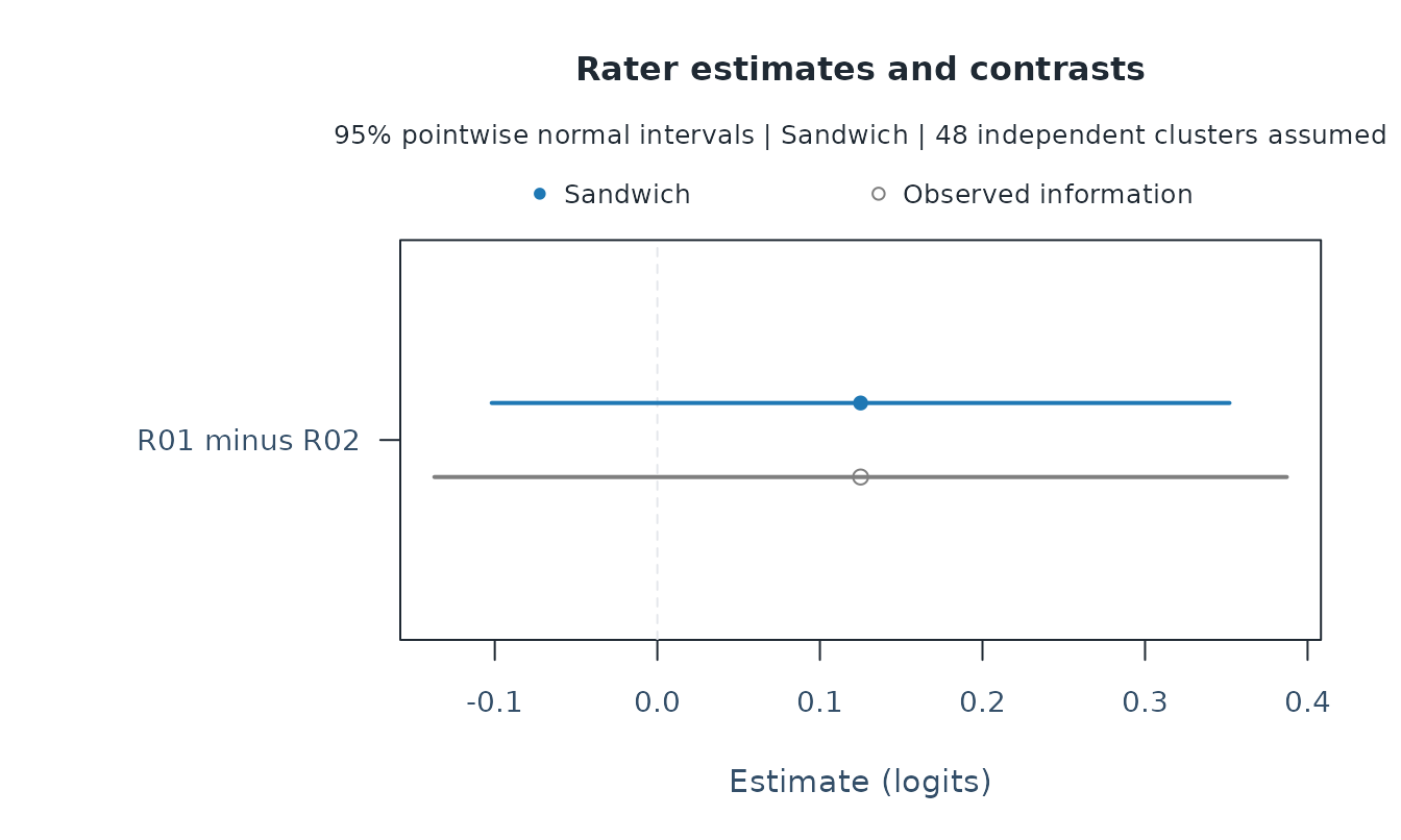

The slight vertical offset distinguishes the methods. Both points have the same horizontal coordinate. The zero line denotes no difference; it is not a threshold of practical importance or a rater-quality rule. Use the size of the difference, interval, rubric and shared rating examples together when giving feedback.

Prepare a sheet for one rater

The functions below answer different practical questions. You can make a figure or a report directly from saved results; neither is required before saving the analysis.

What do you need?	Function and returned object
Retain the fit, diagnostics and chosen intervals together	mfrm_results() returns the analysis object.
Show a saved interval	plot() draws it; as_ggplot() returns a supported ggplot view.
Read an analyst report	mfrm_report() returns a quality-control report by default.
Prepare one recipient’s sheet	mfrm_report(..., style = "rater", output = "html") returns a temporary file path and its content.
Save the complete analysis for later work	saveRDS() writes one R object; export_mfrm_results() writes a folder of selected outputs.

The development version can summarize one rater’s saved results for a feedback conversation. An individual interval and a difference between raters answer different questions: attach ordinary here because it contains each rater’s coefficient. A saved contrast alone cannot become an individual interval.

diagnostics <- diagnose_mfrm(fit, residual_pca = "none")
feedback_results <- mfrm_results(fit, diagnostics = diagnostics,
  intervals = list(raters = ordinary), compute = "never")
sheet <- mfrm_report(feedback_results, style = "rater", facet = "Rater",
  rater = "R01", interval = "raters", output = "html", max_cases = 5)
sheet$report$tables$severity
#>     Severity Reference
#> 1 -0.1838153         0
sheet$report$tables$uncertainty
#>   Level      Lower       Upper Method Available
#> 1  0.95 -0.3447116 -0.02291895  model      TRUE
# Open sheet$path in a browser. Review before copying the HTML file for sharing.

The file contains scoring tendency, its saved interval, exposure, ordinary Infit/Outfit, category use and selected unexpected ratings. It has category-use bars, numerical tables, print styling and no external resources. Set audience = "researcher" for technical guidance, or max_cases = 0 to omit individual cases. Page count depends on the content and print settings.

Choose style for the report’s purpose and output for its format. Omitting style produces an analyst report, and omitting output returns an R object without creating an HTML file. Neither audience = "researcher" nor output = "html" selects a different interval method or confidence level: those choices belong to the earlier mfrm_facet_intervals() call. The default sheet includes up to five unexpected ratings; set max_cases = 0 explicitly if the conversation only needs aggregate summaries.

The default label is “Selected rater”. Other raters’ identities, Person identifiers, task labels and original row numbers are omitted from the sheet and its report object. An explicit label will be displayed. Scores or small groups may still be recognizable, so review the content before sharing. Distribute this standalone HTML file, not the comprehensive results bundle.

The sheet does not refit, recalculate uncertainty, select a warning threshold or decide whether a rater is good or bad. Inspect the full saved interval result and its numerical cautions before preparing the sheet. Missing inputs are explained. If multiple attached interval results contain the selected individual coefficient, choose one explicitly with interval = "raters". GPCM, fitted interactions, imported fits, testlet and shared-random-rater models require their own model-specific reporting routes.

Save the analysis and keep a copy of the sheet

The HTML path is temporary. To keep the sheet after the R session ends, copy the reviewed file to a location you choose. Save the complete analysis separately if you need to prepare another sheet later. The following example uses temporary paths; replace them with your own analysis and recipient-file paths for continuing work.

analysis_file <- tempfile(fileext = ".rds")
saveRDS(feedback_results, analysis_file)
saved_results <- readRDS(analysis_file)

# Reuse the saved diagnostics and intervals for this recipient.
saved_sheet <- mfrm_report(saved_results, style = "rater", facet = "Rater",
  rater = "R01", interval = "raters", output = "html", max_cases = 5)
recipient_file <- tempfile(fileext = ".html")
stopifnot(file.copy(saved_sheet$path, recipient_file, overwrite = FALSE))

The RDS file retains the fitted data and identifiers for the analyst. The recipient HTML contains the selected summaries described above. Copying the HTML does not require sending the RDS file. Reading the saved analysis and preparing another sheet does not rerun estimation or diagnostics; it also does not update an earlier analysis to reflect new ratings.

Carry the same intervals into figures and reports

Suppose the assessment team has chosen a rater difference and its interval method. The figure, table and report should describe that same choice. Attach the saved result instead of calculating a new interval during reporting:

results <- mfrm_results(fit, intervals = list(difference = difference),
                        include = c("fit", "plots"), compute = "never")
apa_table(difference)
#> Fixed-facet uncertainty
#>         Target Estimate   SE Lower Upper ModelSE ModelLower ModelUpper
#>  R01 minus R02     0.13 0.12  -0.1  0.35    0.13      -0.14       0.39
#>     Status Facet   Method ConfidenceLevel Adjustment
#>  available Rater sandwich             95%  Pointwise
#> Note. Pointwise normal intervals conditional on the observed facet levels; changing covariance does not correct biased estimates. Fixed and unavailable targets remain present. No rater-quality decision is implied.
plot_data(results, type = "facet_difference", component = "table")
#>          Target  Estimate        SE      Lower     Upper   ModelSE ModelLower
#> 1 R01 minus R02 0.1250325 0.1157806 -0.1018933 0.3519583 0.1337755 -0.1371626
#>   ModelUpper    Status
#> 1  0.3872276 available
report <- mfrm_report(results)
report$tables$facet_difference_intervals
#>          Target  Estimate        SE      Lower     Upper   ModelSE ModelLower
#> 1 R01 minus R02 0.1250325 0.1157806 -0.1018933 0.3519583 0.1337755 -0.1371626
#>   ModelUpper    Status Facet   Method ConfidenceLevel Adjustment
#> 1  0.3872276 available Rater sandwich             95%  Pointwise

The name difference becomes the plot route facet_difference. A single unnamed result, intervals = difference, uses facet_inference. Several named results can retain different facets, confidence levels or prespecified contrasts. They must all come from the same fitted analysis. A mismatch in data, fitted parameters, constraints, population or integration settings is rejected. An ordinary comparison interval remains separate from the selected sandwich interval, including when the latter is unavailable.

as_ggplot(results, type = "facet_difference", title = NULL, subtitle = NULL,
          preset = "monochrome")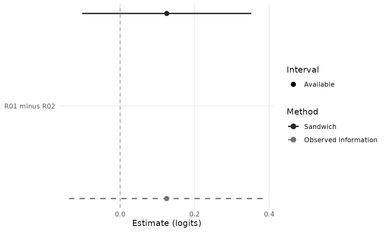

plot(results, type = "facet_difference") uses base graphics; as_ggplot() supports further ggplot customization. Both use the saved values. title = NULL, subtitle = NULL, caption = NULL, reference = NULL and show_legend = FALSE omit the corresponding display parts without changing the stored interval method, level or status. Keep those details in the figure legend or accompanying text when publishing a minimal figure. Shape cues retain unavailable and fixed targets.

summary(results)$reproducible_code shows how to save the complete result and reload it later. In that code, res denotes your result object: use res <- results for this example and choose the file path before saving. Reloading preserves the attached intervals; reconstructing results from fit alone would omit them.

export_mfrm_results(results, ...) includes the selected tables and figures. With preset = "starter", its index.html also links the saved interval figures and describes their methods and confidence levels. When replay is requested, it also saves the RDS and a script that reloads it; replay does not refit the model or recalculate covariance. The settings, contrast coefficients and cluster mapping are retained alongside the interval table. These saved objects contain fitted data and participant identifiers; follow the export function’s data-handling guidance before sharing them.

For an analyst archive with tables, a report and reload instructions, select the components explicitly. include controls files written by the exporter; it does not compute missing analysis components. The folder below retains participant data, which is why this example explicitly acknowledges it.

archive <- export_mfrm_results(feedback_results,
  output_dir = tempfile("rater-analysis-"),
  include = c("tables", "report", "replay", "manifest"),
  acknowledge_sensitive = TRUE)
# Count files by format; inspect archive$written_files for the full index.
table(archive$written_files$Format)
#> 
#>  csv html   md    R  rds 
#>  153    1    1    1    1
archive$plot_errors
#> [1] Plot  Error
#> <0 rows> (or 0-length row.names)
saved_file <- archive$written_files$Path[
  archive$written_files$Component == "results_rds"]
reopened <- readRDS(saved_file)
stopifnot(identical(reopened$facet_intervals, feedback_results$facet_intervals))

Replay also writes the RDS here because the results contain saved intervals. No plots are requested in this example. Add "plots" to export available figures, or use preset = "starter" for the fuller archive. This export preset selects file contents; a plotting preset such as "monochrome" selects appearance. An empty plot_errors table only confirms that no requested plot failed, not that a figure was requested or that the statistical analysis is valid. The report in this archive is the analyst report; use the standalone recipient file created above for the feedback conversation.

This route also works for PCM, whose step structure is declared when fitting:

fit_pcm <- fit_mfrm(ratings, "Person", c("Rater", "Criterion"), "Score",
                    model = "PCM", step_facet = "Criterion", method = "MML")
pcm_difference <- mfrm_facet_intervals(fit_pcm, "Rater", contrasts = contrast,
                                      method = "sandwich", level = 0.90)
pcm_results <- mfrm_results(fit_pcm, intervals = list(difference = pcm_difference),
                            include = c("fit", "plots"), compute = "never")
apa_table(pcm_difference)
#> Fixed-facet uncertainty
#>         Target Estimate   SE Lower Upper ModelSE ModelLower ModelUpper
#>  R01 minus R02     0.13 0.12 -0.07  0.32    0.13      -0.09       0.35
#>     Status Facet   Method ConfidenceLevel Adjustment
#>  available Rater sandwich             90%  Pointwise
#> Note. Pointwise normal intervals conditional on the observed facet levels; changing covariance does not correct biased estimates. Fixed and unavailable targets remain present. No rater-quality decision is implied.

RSM and PCM estimate facet locations while holding discrimination fixed; GPCM slope intervals concern a different target. Attaching a fixed-facet interval does not replace the uncertainty in an ordinary Wright map, alter Infit/Outfit, or provide uncertainty for individual Person scores. Use the facet_ route when you want to display the attached covariance method.

Declare what can be treated as independent

By default, all responses from one person form one sampling unit. A person rated many times does not provide that many independent units. The software first sums their likelihood contributions, then forms the sandwich covariance. Repeated performances by the same person should not be treated as independent merely because they were entered under different IDs.

If persons share a school, clinic or other source of dependence, and those larger clusters can reasonably be treated as independent of one another, supply a person-to-cluster mapping. This fictional mapping only demonstrates the syntax: it is not evidence that the example contains actual schools.

persons <- sort(unique(ratings$Person))
schools <- data.frame(Person = persons,
  Cluster = rep(sprintf("School%02d", 1:16), each = 3))
school_difference <- mfrm_facet_intervals(
  fit, "Rater", contrasts = contrast, method = "sandwich", clusters = schools
)
school_difference$settings[c("persons", "clusters", "cluster_score_rank")]
#> $persons
#> [1] 48
#> 
#> $clusters
#> [1] 16
#> 
#> $cluster_score_rank
#> [1] 8
summary(school_difference)
#>          Target  Estimate        SE      Lower     Upper   ModelSE ModelLower
#> 1 R01 minus R02 0.1250325 0.1236645 -0.1173455 0.3674105 0.1337755 -0.1371626
#>   ModelUpper    Status
#> 1  0.3872276 available

Every fitted person must appear exactly once. Use the column names Person and Cluster in this mapping even if the original data use different names. The number of independent clusters, rather than the number of rating rows, governs the large-sample approximation. Sixteen schools in this illustration are not a recommendation or a demonstrated sufficient sample size.

adjust = TRUE multiplies the covariance by G/(G-1), where G is the number of independent clusters. This simple scaling does not supply a small-sample guarantee or change the normal reference distribution. It is off by default. The user must justify the independence assumption; supplying a mapping does not establish it.

Keep unavailable results visible

When cluster likelihood scores do not span the free-parameter space, the selected sandwich interval is unavailable. The estimate and ordinary comparison remain visible. A fixed anchor has an exact supplied value and no inferential interval; its uncertainty is outside this calculation.

two_groups <- schools
two_groups$Cluster <- rep(c("A", "B"), each = 24)
unavailable <- mfrm_facet_intervals(
  fit, "Rater", contrasts = contrast, method = "sandwich", clusters = two_groups
)
summary(unavailable)[, c("Target", "Estimate", "Lower", "Upper", "Status")]
#>          Target  Estimate Lower Upper                    Status
#> 1 R01 minus R02 0.1250325    NA    NA insufficient_cluster_rank

Increasing the cluster count until this numerical restriction disappears does not establish coverage. A small number of clusters can still yield poor intervals. In plots, a cross marks an unavailable selected interval and an open diamond marks a fixed target. An ordinary comparison interval is never used to replace a missing sandwich interval.

Understand what the sandwich can and cannot address

With many independent units and the required regularity, a sandwich covariance describes variation around the parameter targeted by the fitted working model. If that model is misspecified, this pseudo-true parameter can differ from the generating rater severity. For example, a strongly skewed ability distribution can change the limiting rater difference when the fit insists on a standard normal distribution. Altering the standard error does not remove that shift.

Sparse assignment also needs substantive review. An unassigned rating is not a missing score to fill in; selective assignment can confound rater differences with population differences. Nonresponse depending on an unobserved score is another modeling problem. None of these problems is solved solely by selecting method = "sandwich".

The intervals condition on the observed fixed raters and other facets. They do not describe replacing raters with new draws from a rater population. If shared random rater or task effects span the declared clusters, this one-way independence assumption is inappropriate. The method is not a multiway crossed-cluster estimator. G/D-study planning, variance-component boundaries, EAP person-score uncertainty and multiple-imputation pooling require their own methods. In particular, pool_mfrm_imputed() continues to use its documented within-imputation model covariance; this helper does not change that workflow.

Review quadrature sensitivity separately. The interval helper reuses the fitted integration grid and does not refit the model.

What the bounded simulation showed

A comparison used RSM and PCM, 80 or 320 independent persons, three fixed raters, two criteria and scores from 0 to 2. Each of the eight conditions had 200 independently generated datasets. One scenario used standard-normal ability and six ratings per person. The other combined standardized lognormal ability with three ratings per person; assignment was independent of ability and responses. Thus the second scenario challenges both distribution and design together, without isolating their separate effects.

The comparison evaluated three rater differences and one criterion difference on each same fitted dataset. All 1,600 datasets returned both interval methods. The entries below are ranges across conditions and contrasts, not pooled coverage estimates or confidence bounds. All intervals had a nominal 95% level.

Scenario and reference target	Observed information	Sandwich
Matched normal model: generating truth	92.0–98.0%	92.5–98.0%
Skewed ability and sparse assignment: generating truth	84.5–95.0%	87.0–95.5%
Skewed ability and sparse assignment: working-model target	90.0–97.5%	93.0–97.5%

For example, in the 320-person RSM scenario with skewed ability and sparse assignment, the sandwich covered the generating criterion difference in 87.0% of datasets (95% Monte Carlo interval: 81.5–91.3%). Coverage of the independently calculated working-model target was 96.0% (92.3–98.3%). The same estimates and intervals produced these different answers because the two target values differ. For the R1–R3 difference in the corresponding 320-person PCM scenario, generating-truth coverage was 90.0% (85.0–93.8%). Rater comparisons are therefore subject to this limitation too.

With 200 datasets per condition, Monte Carlo standard error near 95% coverage is about 1.54 percentage points. These results do not demonstrate uniform improvement or a guarantee of nominal coverage. Schools, few independent clusters, shared random raters, informative assignment and nonresponse were not evaluated by this simulation.

Save the analysis and use the plotted data

saved <- tempfile(fileext = ".rds")
saveRDS(difference, saved)
restored <- readRDS(saved)
summary(restored)
#>          Target  Estimate        SE      Lower     Upper   ModelSE ModelLower
#> 1 R01 minus R02 0.1250325 0.1157806 -0.1018933 0.3519583 0.1337755 -0.1371626
#>   ModelUpper    Status
#> 1  0.3872276 available
plotted <- plot(restored, draw = FALSE)
plot_data(plotted)$table
#>          Target  Estimate        SE      Lower     Upper   ModelSE ModelLower
#> 1 R01 minus R02 0.1250325 0.1157806 -0.1018933 0.3519583 0.1337755 -0.1371626
#>   ModelUpper    Status
#> 1  0.3872276 available

The saved result retains the estimates, covariance matrices, likelihood scores, cluster mapping, contrasts, settings and source fit. Printing or plotting it does not fit the model again. Use write.csv(result$table, "intervals.csv", row.names = FALSE) to export a table, and keep the RDS result for its context. Use plot_data() for custom graphics; automatic as_ggplot() conversion is not provided for these method comparisons.

References

The sandwich construction follows the estimating-function framework described by Zeileis (2006). Zeileis, Koell and Graham (2020) discuss clustered covariance estimators and their distinctions. These references support the covariance framework; they do not establish finite-sample accuracy for every MFRM design.