Compare measurement-condition counts in a multivariate D-study

See how a planned change in the number of tasks, raters, or other conditions affects the dependability of a mean score. Plot an existing D-study result; no model is refitted. Start with plot(d) for G and Phi, then use plot(d, type = "sem") to examine error in score units. If the result has several composites, select one explicitly with composite.

Usage

# S3 method for class 'mfrm_multivariate_d_study'
plot(
  x,
  type = c("coefficients", "sem"),
  score = NULL,
  x_var = NULL,
  draw = TRUE,
  preset = "standard",
  composite = NULL,
  ...
)

Arguments

x: A result from mfrm_multivariate_d_study().
type: "coefficients" shows G and Phi in separate panels; "sem" shows relative and absolute standard errors of measurement.
score: A single original score name. An explicit name always selects an original score, even if a composite has the same name. If both score and composite are NULL, select the sole composite, or the first score when there are no composites. Several composites require an explicit selection. The title identifies the selection and any composite weights. Call the method again to inspect another score or composite.
x_var: A count column in x$design_grid: "Tasks"/"Raters" for the task/rater interface, or a facet label supplied through facets. By default use the last varying count column, or the last column if none varies. A one-facet result permits only its included facet. Each line holds the other facet count constant.
draw: Draw the plot when TRUE; FALSE only returns its data.
preset: Plot style: "standard", "publication", "compact", or "monochrome". Point shapes and line types also distinguish counts.
composite: A single composite name from x$coefficients, as defined by a weight-matrix column, or "Composite" for vector weights. Supply either score or composite, not both.
...: Reserved for future use; additional arguments are rejected.

Value

Invisibly, an mfrm_plot_data object. Use plot_data() to extract table (the selected score/composite), series (one row per scenario and plotted metric, including missing values), unavailable, design_grid, weights, score identity, axis/group names, labels, component_note, and legend settings. In series, Status is specific to Metric; table retains the original row status and metric-specific columns. weights contains the selected composite's named weight vector, or NULL when plotting an original score. as_ggplot() preserves these comparisons for editing or export with the optional ggplot2 package; for example, as_ggplot(d, type = "sem").

Details

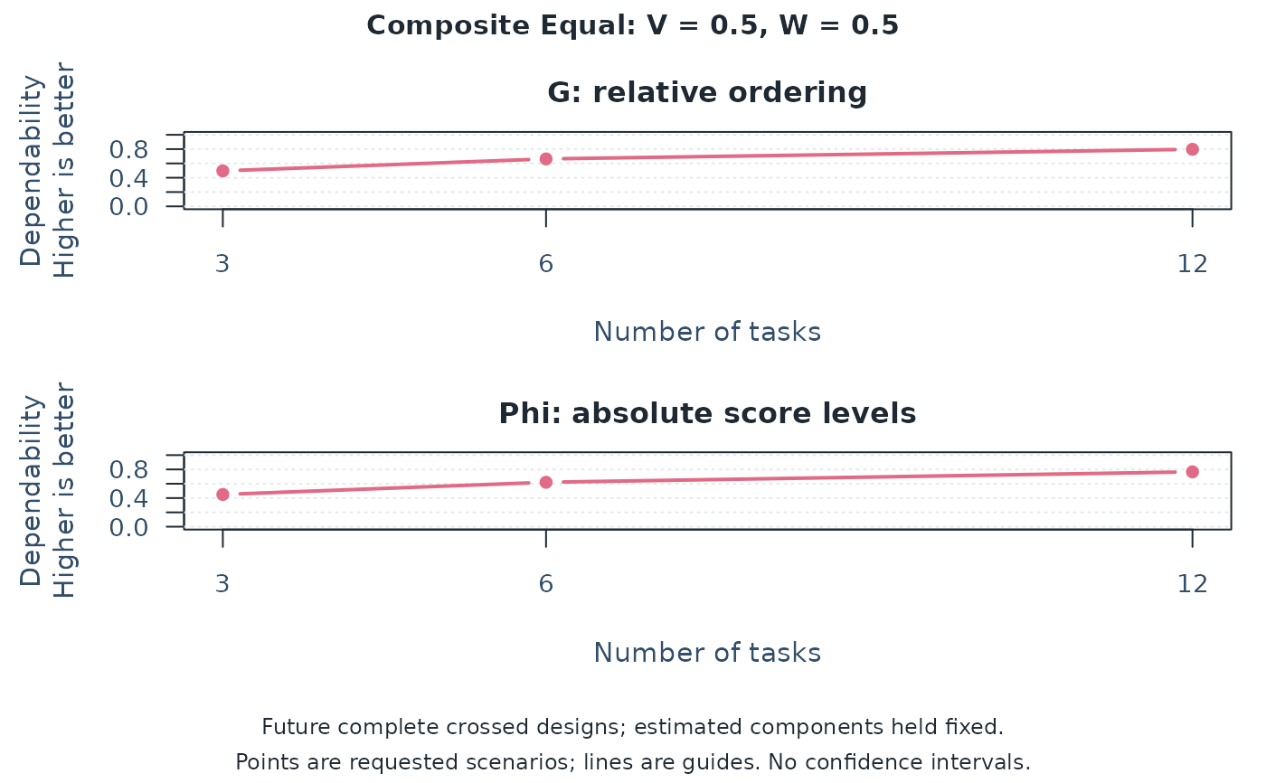
G describes consistency of relative ordering: for example, ranking examinees. Phi also includes shifts caused by easier tasks or more lenient raters and concerns absolute score levels. Higher coefficients indicate greater dependability under the fitted model; neither gives the probability of a correct pass/fail decision. No universal acceptable cutoff is drawn.

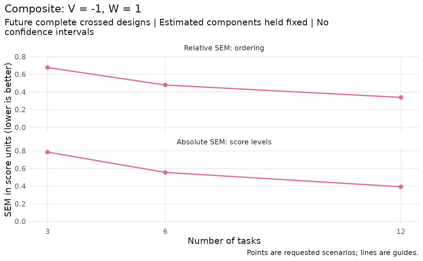
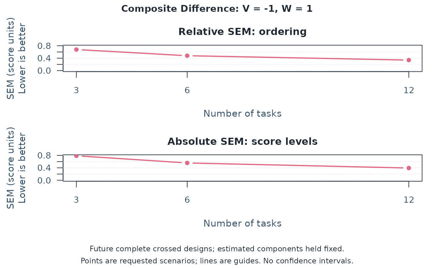
SEM is the square root of error variance. Lower values indicate less error in the units of the selected mean score or composite. Relative SEM concerns ordering; absolute SEM also includes condition-wide shifts. SEM is not a confidence interval for G or Phi. The two SEM panels share a scale, but different scores or differently scaled composites need not have comparable units. Weights are not normalized. Changing weights can also change the meaning of the score; a higher G or Phi alone does not justify a new set of weights.

Points represent only the supplied scenarios. Lines connect them as visual guides within a fixed count of the other facet, without fitting a curve or evaluating intermediate designs. For example, with tasks on the horizontal axis, compare points along one line to change tasks while keeping raters constant. Compare lines at the same task count to change raters.

Multivariate means several score criteria, not a requirement for a 3D plot. Use these 2D panels to compare counts while holding the other facet fixed. With many lines, specify a smaller set of relevant plans when creating the D-study and inspect scores/composites separately. This method does not draw a heatmap or 3D surface. For uncertainty in a prespecified change, use mfrm_multivariate_d_compare() and its plot method; an SEM curve is not a confidence band. plot_data() supplies exact values, including unavailable estimates, and preset = "monochrome" retains line/point distinctions.

Coefficients also depend on variation among persons. If universe-score variance increases while error variance stays constant, G and Phi increase but SEM does not decrease. Therefore, comparing coefficients across different populations does not isolate improvement in the assessment. Read the SEMs, score units and target population alongside the coefficients.

Scenarios retain the G-study's crossed or nested structure, with complete balanced future conditions shared by every person and score. For a nested facet, the axis or legend says "per" to identify its count within each parent, for example "Raters per Task"; this is not the total rater pool size. Even when the G-study used incomplete data, the figure does not describe reliability of that sparse roster. Projections hold estimated covariance components fixed and have no sampling confidence intervals. A flattening curve can indicate limited gains from adding one facet alone; it does not identify a cost-effective optimum. The highest point alone does not account for uncertainty in the estimated components. Read the size of differences as well as their ordering. Equal products of rater and task counts give equal rating counts, not necessarily equal examinee burden or total cost. Unavailable candidates prevent a complete comparison for that metric.

Unavailable estimates stay missing. A panel with no estimates states the reason; otherwise a margin note reports unavailable scenarios. The returned unavailable table preserves their counts, metrics, and Status values. Each panel uses its metric's status, so an unavailable Phi does not hide an available G. Non-PSD component matrices are noted separately on the figure; inspect x$component_diagnostics before using raw projections. Increasing planned counts does not repair those component estimates. Missing values are never plotted as zero. Previously saved D-study objects retain their recorded values and availability: rerun mfrm_multivariate_d_study() on the saved G-study to apply current rules.

Session plot defaults

Set options(mfrmr.plot_preset = "publication") to choose a session default for plotting functions that expose the common preset argument. The supported values are "standard", "publication", "compact" and "monochrome". Precedence is an explicit call argument, then the session option, then "standard". For example, preset = "standard" overrides a session set to "monochrome". Explicit preset = NULL retains the earlier package-default behavior; it does not read the session option. Invalid session values cause an error only when that option is needed.

The category-curve, data-quality, fit-review, connectivity and network routes of plot() for report bundles use the same option through .... Plots without a common preset argument, including extended-model plots with their own palette controls, keep their own settings. This option selects a preset, not a universal theme or a guarantee that all renderers implement every appearance control identically.

New plot payloads retain the resolved preset for supported saved-data rendering. Converting an existing payload with as_ggplot() uses its saved appearance, even after the session option changes. A call that creates a new plot from a fit or statistical result uses the current default. For a reproducible script, supply preset explicitly or set the option in that script. Saving only the fitted model does not save a session option. No global ggplot theme is changed.

Restore previous settings with old <- options(mfrmr.plot_preset = "monochrome") followed by options(old). Use options(mfrmr.plot_preset = NULL) to remove the option. The preset changes appearance, not estimates, confidence levels or diagnostic thresholds.

Examples

# Question: how much would doubling the common tasks change dependability?
tasks <- read.csv(system.file("extdata", "mgenova-table12.csv", package = "mfrmr"))
g <- mfrm_multivariate_gstudy(tasks, c("V", "W"), rater = NULL)
d <- mfrm_multivariate_d_study(g, data.frame(Tasks = c(3, 6, 12)),
  weights = c(V = -1, W = 1))
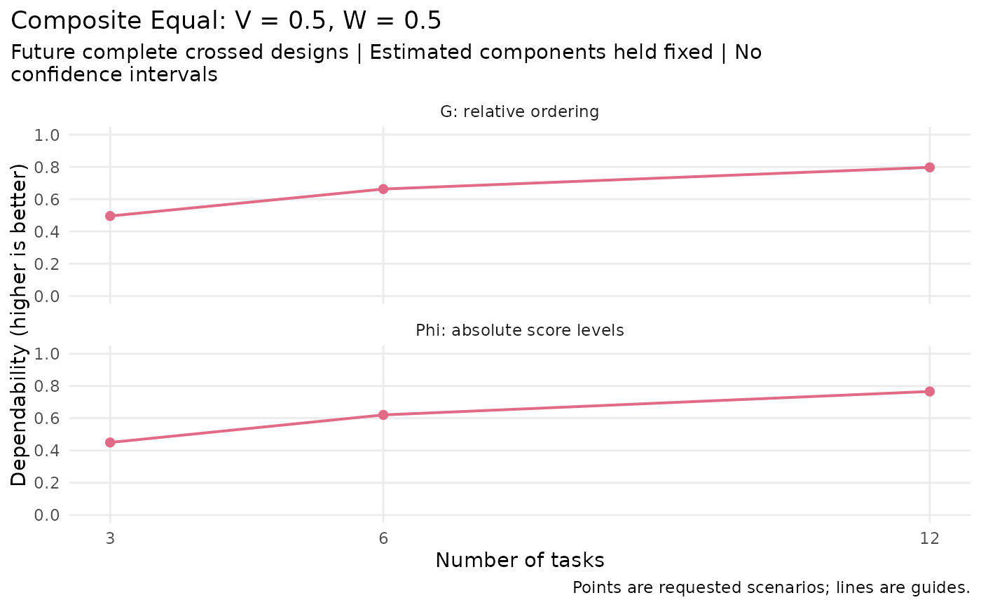
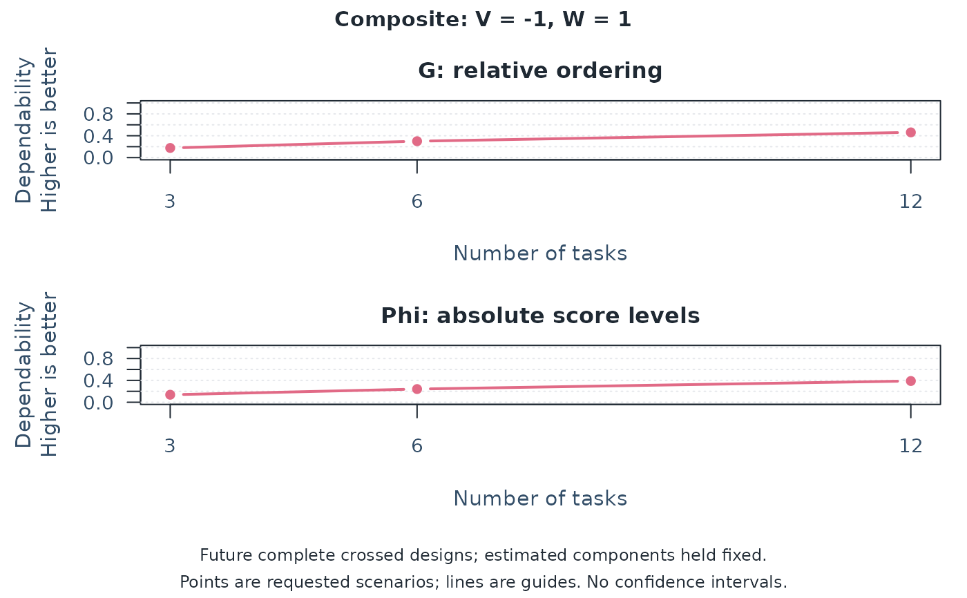
plot(d) # Default: the difference W minus V; higher G/Phi is better.

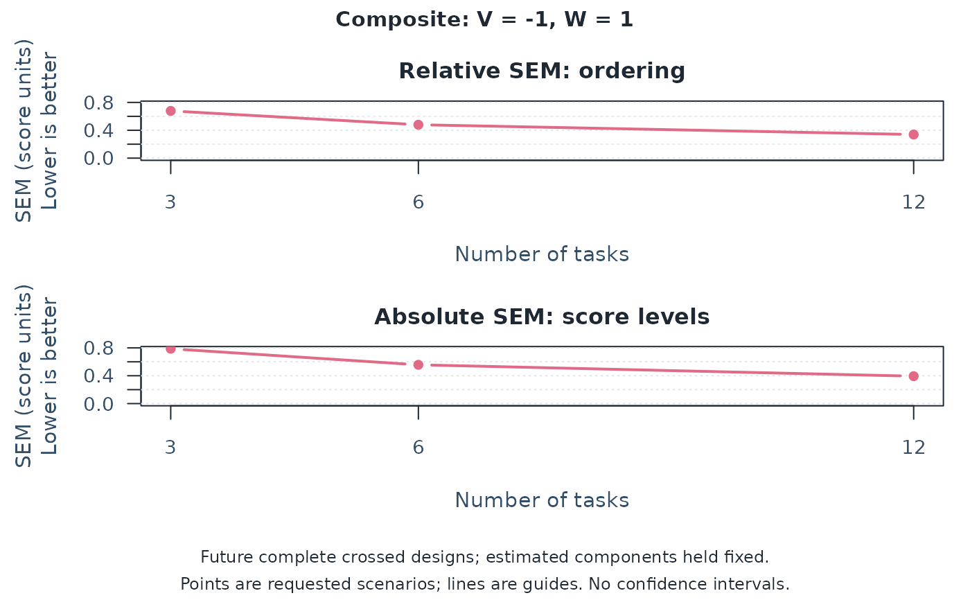
plot(d, type = "sem") # Error in difference-score units; lower is better.

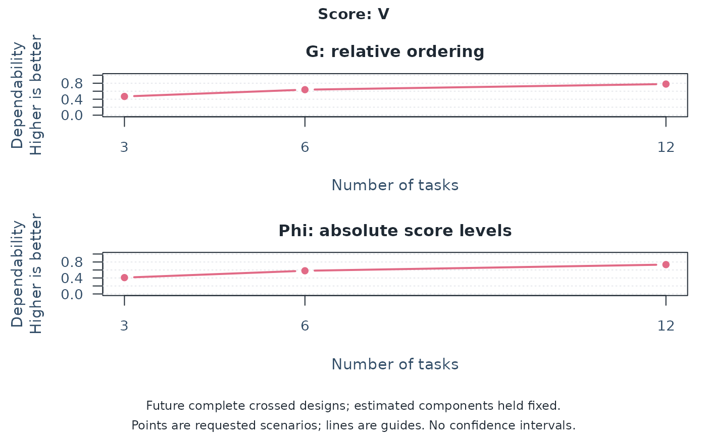
plot(d, score = "V") # Inspect an original score separately.

values <- plot_data(plot(d, draw = FALSE))
values$table # Exact values and availability, rather than reading off a line.
#>   Scenario Tasks      Kind     Score UniverseVariance RelativeErrorVariance
#> 3        1     3 Composite Composite       0.09851852             0.4597531
#> 6        2     6 Composite Composite       0.09851852             0.2298765
#> 9        3    12 Composite Composite       0.09851852             0.1149383
#>   AbsoluteErrorVariance         G       Phi RelativeSEM AbsoluteSEM    Status
#> 3                 0.620 0.1764706 0.1371134   0.6780509   0.7874008 Available
#> 6                 0.310 0.3000000 0.2411605   0.4794544   0.5567764 Available
#> 9                 0.155 0.4615385 0.3886048   0.3390255   0.3937004 Available
#>     GStatus PhiStatus RelativeSEMStatus AbsoluteSEMStatus ComponentPSD
#> 3 Available Available         Available         Available         TRUE
#> 6 Available Available         Available         Available         TRUE
#> 9 Available Available         Available         Available         TRUE
if (requireNamespace("ggplot2", quietly = TRUE)) {
  p <- as_ggplot(d, type = "sem")
  print(p)
  # ggplot2::ggsave("d-study-sem.png", p, width = 7, height = 7, dpi = 300)
}


# A weight matrix names several choices; explicitly select the plotted one.
alternatives <- mfrm_multivariate_d_study(g, data.frame(Tasks = c(3, 6, 12)),
  weights = cbind(Equal = c(V = 0.5, W = 0.5), Difference = c(V = -1, W = 1)))
plot(alternatives, composite = "Equal")

plot(alternatives, composite = "Difference", type = "sem")

if (requireNamespace("ggplot2", quietly = TRUE)) {
  print(as_ggplot(alternatives, composite = "Equal"))
}