
plot_data() is a small accessor for users who want to build custom
base-R, ggplot2, plotly, or table-based displays from mfrmr plot helpers.
It accepts an existing mfrm_plot_data object, or any mfrmr object whose
plot() method supports draw = FALSE. Use plot_data_components() first
when you want to inspect which components are available before extracting
one.
Arguments
- x
An
mfrm_plot_dataobject, or a fitted/report/review object with aplot(..., draw = FALSE)method.- component
Optional single component name inside the reusable plot data. When
NULL, the full plot-data list is returned.- type
Optional plot type passed to
plot()whenxis not already anmfrm_plot_dataobject.- ...
Additional arguments passed to
plot(..., draw = FALSE)whenxis not already anmfrm_plot_dataobject.
Examples
# \donttest{
# Load the package and example ratings
library(mfrmr)
toy <- load_mfrmr_data("example_operational")
# Fit the model
fit <- fit_mfrm(
data = toy,
person = "Person",
facets = c("Rater", "Criterion"),
score = "Score",
method = "MML",
model = "RSM"
)
# Draw the Wright map and keep its reusable data
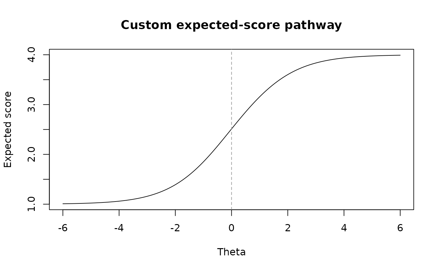
wright <- plot(fit)
 # Extract the plotted locations as a table
locations <- plot_data(wright, component = "locations")
head(locations)
#> # A tibble: 6 × 38
#> Group Label PlotType Estimate SE Fixed CI_Level SE_Method PrecisionTier
#> <fct> <chr> <chr> <dbl> <dbl> <lgl> <dbl> <chr> <chr>
#> 1 Rater R01 Facet level -0.606 0.181 FALSE 0.95 Observati… exploratory
#> 2 Rater R02 Facet level -0.382 0.166 FALSE 0.95 Observati… exploratory
#> 3 Rater R04 Facet level 0.180 0.185 FALSE 0.95 Observati… exploratory
#> 4 Rater R05 Facet level 0.184 0.199 FALSE 0.95 Observati… exploratory
#> 5 Rater R03 Facet level 0.212 0.179 FALSE 0.95 Observati… exploratory
#> 6 Rater R06 Facet level 0.412 0.219 FALSE 0.95 Observati… exploratory
#> # ℹ 29 more variables: SupportsFormalInference <lgl>, SEUse <chr>,
#> # CIBasis <chr>, CIUse <chr>, CIEligible <lgl>, CILabel <chr>,
#> # Measure_Source <chr>, CI_Lower <dbl>, CI_Upper <dbl>, Step <chr>,
#> # StepIndex <int>, BoundarySeparated <lgl>, XBase <dbl>, X <dbl>,
#> # OriginalEstimate <dbl>, BelowRange <lgl>, AboveRange <lgl>,
#> # DisplayEstimate <dbl>, DisplayLabel <chr>, OriginalCI_Lower <dbl>,
#> # OriginalCI_Upper <dbl>, DisplayCI_Lower <dbl>, DisplayCI_Upper <dbl>, …
# For table extraction alone, no graphics device is needed
locations_only <- plot_data(fit, component = "locations")
head(locations_only)
#> # A tibble: 6 × 38
#> Group Label PlotType Estimate SE Fixed CI_Level SE_Method PrecisionTier
#> <fct> <chr> <chr> <dbl> <dbl> <lgl> <dbl> <chr> <chr>
#> 1 Rater R01 Facet level -0.606 0.181 FALSE 0.95 Observati… exploratory
#> 2 Rater R02 Facet level -0.382 0.166 FALSE 0.95 Observati… exploratory
#> 3 Rater R04 Facet level 0.180 0.185 FALSE 0.95 Observati… exploratory
#> 4 Rater R05 Facet level 0.184 0.199 FALSE 0.95 Observati… exploratory
#> 5 Rater R03 Facet level 0.212 0.179 FALSE 0.95 Observati… exploratory
#> 6 Rater R06 Facet level 0.412 0.219 FALSE 0.95 Observati… exploratory
#> # ℹ 29 more variables: SupportsFormalInference <lgl>, SEUse <chr>,
#> # CIBasis <chr>, CIUse <chr>, CIEligible <lgl>, CILabel <chr>,
#> # Measure_Source <chr>, CI_Lower <dbl>, CI_Upper <dbl>, Step <chr>,
#> # StepIndex <int>, BoundarySeparated <lgl>, XBase <dbl>, X <dbl>,
#> # OriginalEstimate <dbl>, BelowRange <lgl>, AboveRange <lgl>,
#> # DisplayEstimate <dbl>, DisplayLabel <chr>, OriginalCI_Lower <dbl>,
#> # OriginalCI_Upper <dbl>, DisplayCI_Lower <dbl>, DisplayCI_Upper <dbl>, …
# }
# Extract the plotted locations as a table
locations <- plot_data(wright, component = "locations")
head(locations)
#> # A tibble: 6 × 38
#> Group Label PlotType Estimate SE Fixed CI_Level SE_Method PrecisionTier
#> <fct> <chr> <chr> <dbl> <dbl> <lgl> <dbl> <chr> <chr>
#> 1 Rater R01 Facet level -0.606 0.181 FALSE 0.95 Observati… exploratory
#> 2 Rater R02 Facet level -0.382 0.166 FALSE 0.95 Observati… exploratory
#> 3 Rater R04 Facet level 0.180 0.185 FALSE 0.95 Observati… exploratory
#> 4 Rater R05 Facet level 0.184 0.199 FALSE 0.95 Observati… exploratory
#> 5 Rater R03 Facet level 0.212 0.179 FALSE 0.95 Observati… exploratory
#> 6 Rater R06 Facet level 0.412 0.219 FALSE 0.95 Observati… exploratory
#> # ℹ 29 more variables: SupportsFormalInference <lgl>, SEUse <chr>,
#> # CIBasis <chr>, CIUse <chr>, CIEligible <lgl>, CILabel <chr>,
#> # Measure_Source <chr>, CI_Lower <dbl>, CI_Upper <dbl>, Step <chr>,
#> # StepIndex <int>, BoundarySeparated <lgl>, XBase <dbl>, X <dbl>,
#> # OriginalEstimate <dbl>, BelowRange <lgl>, AboveRange <lgl>,
#> # DisplayEstimate <dbl>, DisplayLabel <chr>, OriginalCI_Lower <dbl>,
#> # OriginalCI_Upper <dbl>, DisplayCI_Lower <dbl>, DisplayCI_Upper <dbl>, …
# For table extraction alone, no graphics device is needed
locations_only <- plot_data(fit, component = "locations")
head(locations_only)
#> # A tibble: 6 × 38
#> Group Label PlotType Estimate SE Fixed CI_Level SE_Method PrecisionTier
#> <fct> <chr> <chr> <dbl> <dbl> <lgl> <dbl> <chr> <chr>
#> 1 Rater R01 Facet level -0.606 0.181 FALSE 0.95 Observati… exploratory
#> 2 Rater R02 Facet level -0.382 0.166 FALSE 0.95 Observati… exploratory
#> 3 Rater R04 Facet level 0.180 0.185 FALSE 0.95 Observati… exploratory
#> 4 Rater R05 Facet level 0.184 0.199 FALSE 0.95 Observati… exploratory
#> 5 Rater R03 Facet level 0.212 0.179 FALSE 0.95 Observati… exploratory
#> 6 Rater R06 Facet level 0.412 0.219 FALSE 0.95 Observati… exploratory
#> # ℹ 29 more variables: SupportsFormalInference <lgl>, SEUse <chr>,
#> # CIBasis <chr>, CIUse <chr>, CIEligible <lgl>, CILabel <chr>,
#> # Measure_Source <chr>, CI_Lower <dbl>, CI_Upper <dbl>, Step <chr>,
#> # StepIndex <int>, BoundarySeparated <lgl>, XBase <dbl>, X <dbl>,
#> # OriginalEstimate <dbl>, BelowRange <lgl>, AboveRange <lgl>,
#> # DisplayEstimate <dbl>, DisplayLabel <chr>, OriginalCI_Lower <dbl>,
#> # OriginalCI_Upper <dbl>, DisplayCI_Lower <dbl>, DisplayCI_Upper <dbl>, …
# }