Build an unexpected-response screening report

Usage

unexpected_response_table(
  fit,
  diagnostics = NULL,
  abs_z_min = 2,
  prob_max = 0.3,
  top_n = 100,
  rule = c("either", "both")
)

Arguments

fit: Output from fit_mfrm().
diagnostics: Optional output from diagnose_mfrm().
abs_z_min: Absolute standardized-residual cutoff.
prob_max: Maximum observed-category probability cutoff.
top_n: Maximum number of ranked rows to return in table. Summary counts and percentages always use all flagged observations.
rule: Flagging rule: "either" (default) or "both".

Value

A named list with:

table: flagged response rows
summary: one-row overview
thresholds: applied thresholds

Details

A response is flagged as unexpected when:

rule = "either": |StdResidual| >= abs_z_min OR ObsProb <= prob_max
rule = "both": both conditions must be met.

Missing inputs preserve an unavailable rule outcome unless the other condition determines the result (for example, a true condition suffices for either). Summaries retain evaluated and unavailable counts; the full-sample percentage is withheld if any outcome is unavailable.

The table includes row-level observed/expected values, residuals, observed-category probability, most-likely category, and a composite severity score for sorting.

Interpreting output

summary: prevalence of unexpected responses under current thresholds, before limiting the displayed rows with top_n.
table: ranked row-level diagnostics for case review.
thresholds: active cutoffs and flagging rule.

Compare results across rule = "either" and rule = "both" to assess how conservative your screening should be.

Typical workflow

Start with rule = "either" for broad screening.
Re-run with rule = "both" for strict subset.
Inspect top rows and visualize with plot_unexpected().

Further guidance

For a plot-selection guide and a longer walkthrough, see mfrmr_visual_diagnostics and vignette("mfrmr-visual-diagnostics", package = "mfrmr").

Output columns

The table data.frame contains:

Row: Original row index in the prepared data.
Person: Person identifier (plus one column per facet).
Score: Observed score category.
Observed, Expected: Observed and model-expected score values.
Residual, StdResidual: Raw and standardized residuals.
ObsProb: Probability of the observed category under the model.
MostLikely, MostLikelyProb: Most probable category and its probability.
Severity: Composite severity index (higher = more unexpected).
Direction: "Higher than expected" or "Lower than expected".
FlagLowProbability, FlagLargeResidual: Logical flags for each criterion.

The summary data.frame contains:

TotalObservations: Total observations analyzed.
UnexpectedN, UnexpectedPercent: Known flagged count and full-sample percentage. The percentage is unavailable when any rule outcome is unknown; the count is unavailable when no response can be evaluated.
EvaluatedObservations, UnavailableObservations: Responses whose rule outcome is determined or unavailable.
AbsZThreshold, ProbThreshold: Applied cutoff values.
Rule: "either" or "both".

Examples

# \donttest{
library(mfrmr)
toy <- load_mfrmr_data("example_operational")
fit <- fit_mfrm(
  data = toy,
  person = "Person",
  facets = c("Rater", "Criterion"),
  score = "Score",
  method = "MML",
  model = "RSM"
)
diagnostics <- diagnose_mfrm(fit)
unexpected <- unexpected_response_table(
  fit, diagnostics = diagnostics, abs_z_min = 1.5, prob_max = 0.4, top_n = 5
)
unexpected$summary # Counts and percentages for all flagged observations
#> # A tibble: 1 × 10
#>   TotalObservations EvaluatedObservations UnavailableObservations UnexpectedN
#>               <int>                 <int>                   <int>       <int>
#> 1               282                   282                       0         141
#> # ℹ 6 more variables: UnexpectedPercent <dbl>, LowProbabilityN <int>,
#> #   LargeResidualN <int>, Rule <chr>, AbsZThreshold <dbl>, ProbThreshold <dbl>
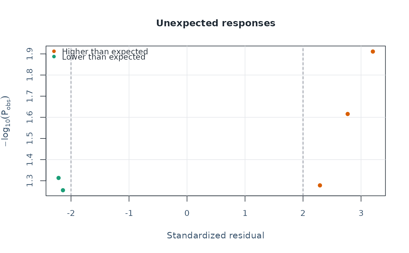
unexpected$table   # Only the five highest-ranked cases
#>   Row Person Rater    Criterion Weight Score Observed Expected  Residual
#> 1  90   P016   R02 Organization      1     4        4 1.712717  2.287283
#> 2  69   P012   R03 Organization      1     4        4 1.881621  2.118379
#> 3 282   P048   R06 Organization      1     4        4 2.126046  1.873954
#> 4 121   P021   R04      Content      1     1        1 2.867349 -1.867349
#> 5 145   P025   R04     Language      1     1        1 2.815285 -1.815285
#>   StdResidual    ObsProb MostLikely MostLikelyProb CategoryGap Surprise
#> 1    3.204010 0.01227149          2      0.4446563           2 1.911103
#> 2    2.769635 0.02422218          2      0.4736443           2 1.615787
#> 3    2.291484 0.05270294          2      0.4734400           2 1.278165
#> 4   -2.214482 0.04860959          3      0.4171721           2 1.313278
#> 5   -2.139004 0.05557605          3      0.4123865           2 1.255112
#>              Direction FlagLowProbability FlagLargeResidual Severity
#> 1 Higher than expected               TRUE              TRUE 6.115113
#> 2 Higher than expected               TRUE              TRUE 5.385422
#> 3 Higher than expected               TRUE              TRUE 4.569650
#> 4  Lower than expected               TRUE              TRUE 4.527760
#> 5  Lower than expected               TRUE              TRUE 4.394117
plot(unexpected)

# The rule is exploratory: inspect the scoring context before changing a rating
# }