mfrmr Workflow and Method Map

Start with one analysis: load ratings, fit a model, plot the results, and read the summary. The Examples section contains a complete runnable script. The later sections describe diagnostics, reporting, and specialist routes.

Start here

Load the package with library(mfrmr) and example ratings with toy <- load_mfrmr_data("example_operational").
Fit with fit_mfrm(). The person, facets, and score arguments name columns in the data; each row represents one rating event.
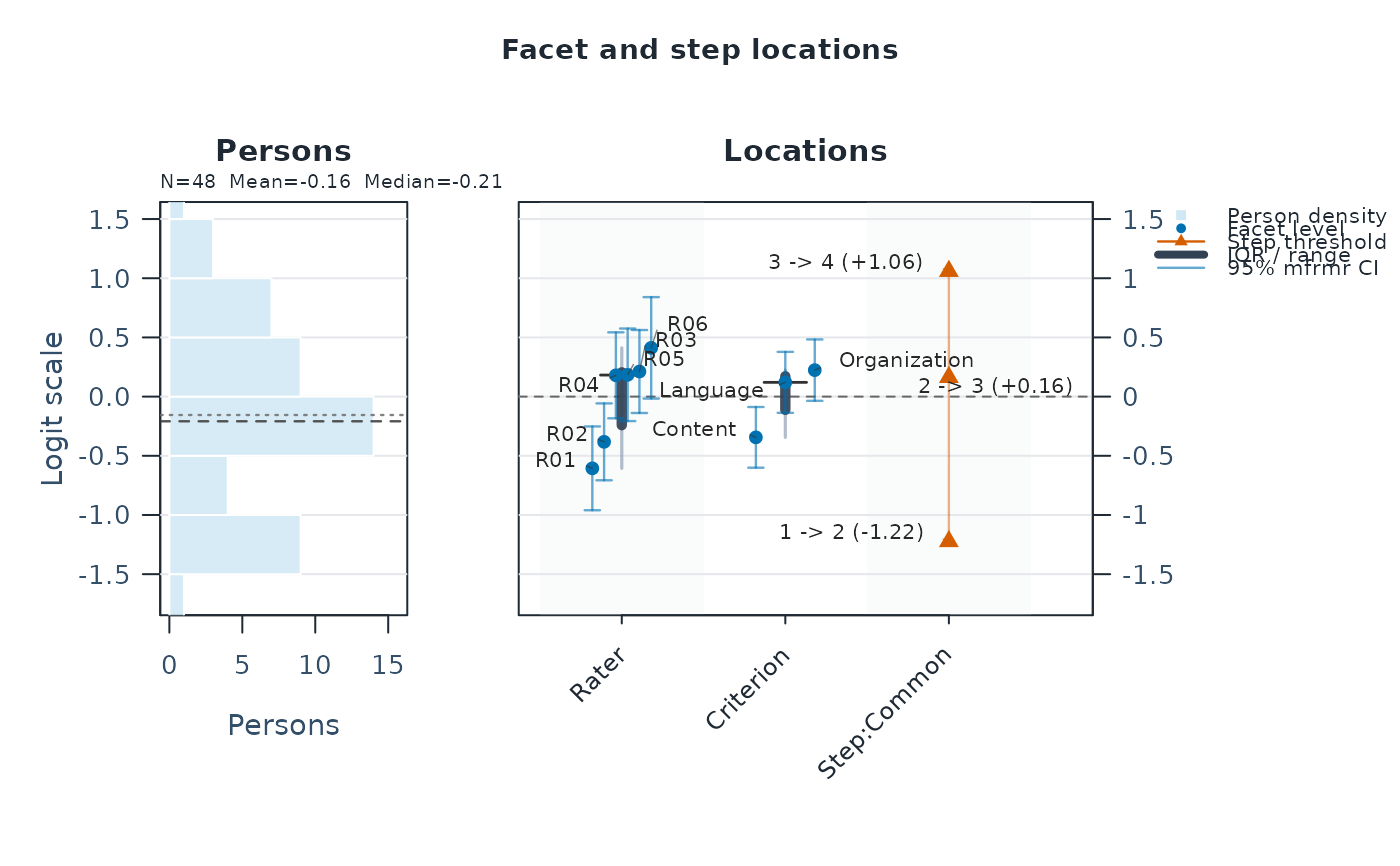
Draw the Wright map with plot(fit) to view person abilities, rater severities, criterion difficulties, and category thresholds together.
Save results <- summary(fit) and inspect results$person_overview and results$facet_overview for the distributions of estimates.

These overview tables summarize distributions. Use as.data.frame(fit) for individual person, rater, and criterion estimates, identified by Facet and Level. Before interpreting or reporting estimates, read results$decision and follow its NextAction; the default summary does not compute diagnostics. For your own data, first check the rating design and score categories with describe_mfrm_data(). head(toy) shows the input rows; Study and Group are extra labels unused by this model. <- saves an object and $ selects a named part of it.

From the first summary to diagnostics

A FormalInference = "No" entry in results$decision can mean that precision has not yet been reviewed. Read Why and NextAction to distinguish that state from a detected problem. Run diagnostics <- diagnose_mfrm(fit) and inspect summary(diagnostics)$decision. To reuse these checks in the fuller reporting object, call res <- mfrm_results(fit, diagnostics = diagnostics). Here results is the basic summary and res is the comprehensive object accepted by mfrm_report() and export_mfrm_results().

Understand the function names

Learn the operation first, then open its help page:

fit_ estimates model parameters, for example fit_mfrm().
score_ estimates Person abilities using a fitted calibration, for example score_mfrm_persons() for people already in a supported fitted RSM.
pool_ combines eligible analyses, for example pool_mfrm_imputed().
review_ checks supplied data or analysis choices, for example review_mfrm_imputations(); it does not generate missing scores.
export_ writes files, for example export_mfrm_results().
summary(object) and plot(object) select a method for the object you supply. You normally do not call plot.mfrm_testlet() directly.

The package name is mfrmr; mfrm in analysis functions refers to a many-facet Rasch model. Some help guides use the package prefix mfrmr_. The prefixes do not select different estimators. For a short ordinary-MFRM map, use mfrmr_output_guide("beginner")[, c("Question", "MainFunction")]. The no-argument guide lists all specialist routes and is not a first lesson. For rater feedback, use mfrmr_output_guide("feedback"): it distinguishes uncertainty in severity from unexpected rating patterns and the accuracy of a warning rule. mfrm_facet_intervals() concerns specified fixed raters; shared-rater intervals have a different target and retain their separate limitations. Ordinary and extended-model residuals also use different definitions. The guide names the matching summary, plot and saving routes.

review_mfrm_imputations() checks completed data supplied by you; it does not generate missing scores. Follow it with fit_mfrm_imputed() and then pool_mfrm_imputed(). mfrm_screening_performance() evaluates a warning rule against known simulation truth. mfrm_screening_sensitivity() repeats that evaluation across specified thresholds; it does not establish accuracy from real ratings alone. mfrm_pca() summarizes numeric external attributes; mfrm_cluster_kmeans() forms groups. PCA is optional before k-means. mfrm_cluster_pam() uses partitioning around medoids (PAM) for mixed attributes; it does not automatically choose a clustering algorithm. For a dendrogram, use mfrm_cluster_hierarchical(). A G-study (mfrm_multivariate_gstudy()) estimates sources of variation in observed scores; a D-study (mfrm_multivariate_d_study()) uses them to compare future rater/task plans. Neither needs an MFRM fit.

Updating earlier scripts

Earlier call	Recommended call	Meaning retained
`mfrm_cluster(x, k)`	`mfrm_cluster_pam(x, k)`	Same Gower/PAM partition and result class.
`mfrm_response_imputations(..., impute = ids)`	`review_mfrm_imputations(..., impute_ids = ids)`	Same checks of supplied completed ratings; no imputation model is fitted.
`keep_original = TRUE`	`category_policy = "preserve"`	Same category ladder in fitting, data review and anchor review.
`keep_original = FALSE`	`category_policy = "collapse"`	Same collapsing of gaps; still the default when no policy is supplied.

The old calls remain supported, including positional arguments. Saved objects retain their classes and summary()/plot() methods. Do not pass conflicting old/new category choices. See compatibility_alias_table() for the complete migration map. This does not change what predict() returns: use the ability-scoring or response-prediction route named for your model.

A calibration is the fitted set of model parameters, such as rater severity and category thresholds. A conditional ability interval holds them fixed; it excludes uncertainty from estimating the calibration. EAP is the mean of the conditional ability distribution. An SE describes uncertainty in an estimate; an SD describes spread. Check whether an SD refers to differences among persons or one Person's posterior.

Check defaults before adapting an example

An omitted argument selects a convention, not the best choice for your assessment. Start with the choices that change the analysis:

Model and population: fit_mfrm() defaults to RSM and MML. RSM uses shared category thresholds. With PCM, set step_facet explicitly instead of relying on facet-name inference or the first-facet fallback. Ordinary RSM/PCM MML with population_formula = NULL fixes the ability distribution at N(0,1). Both extended RSMs instead estimate ability variance by default (person_sd = NULL). Their model-comparison tutorials show how to match population assumptions. Changing only the fitting function can change more than the rater/dependence structure.
Estimator choice: MML is the current default, not the result of an automatic comparison of estimators. It uses a population model for abilities. JML estimates each person's ability as a separate parameter; it does not fit a population distribution during calibration. Choosing JML does not automatically correct the bias associated with few ratings per person. Without jml_correction_order, JML is uncorrected and its location SEs are exploratory. Shared-owner GPCM also supports an explicit, experimental correction order. Its RootSE describes local variation around the adjusted-equation root; residual bias may remain and structural confidence intervals are not supplied. See the estimator discussion in fit_mfrm(). Neither a larger model nor a smaller reported SE establishes a better analysis. Choose from the assessment question, rating design and modeling assumptions, rather than from whether the user is a beginner or expert.
Rating scale: supply rating_min, rating_max and category_policy from the rubric in both data review and ordinary fitting. Omitted bounds use the observed range. The ordinary default category_policy = NULL retains keep_original = FALSE and can collapse unobserved internal categories, for example observed 1, 3, 5 to 1, 2, 3. This changes the fitted category structure, not just labels. A warning and the stored score map identify the recoding. Inspect CategoryPolicy and ScoreRecoded in data_review$overview or summary(fit)$settings_overview to distinguish the chosen rule from an actual change to score values. With a complete contiguous scale, "collapse" can still have ScoreRecoded = FALSE. Use category_policy = "preserve" to preserve the declared ladder; an unsupported internal category then stops fitting and needs substantive review.
Missingness and assignment: ordinary fitting excludes rows missing a score or required ID (and nonpositive-weight rows); inspect fit$prep$row_retention, fit$prep$preparation_notes and fit$prep$score_map. Missing-code conversion is off unless requested. In contrast, the extended models stop on missing assigned scores by default, and feature/G-study routes also require an explicit omission choice. Omission does not correct informative missingness. In review_mfrm_imputations(), assigned = NULL declares every supplied row assigned: supply an assignment column if unassigned rows are present.
Included effects: both extensions default to no additional fixed facets. For example, testlet = "Task" groups local dependence but does not itself add fixed task difficulty; request that with facets = "Task" when it is part of the intended model.
Feature geometry: PCA and direct k-means default to scale = TRUE and equal feature weights. Thus years of experience and hours of training contribute in SD units; scale = FALSE retains their measurement units. PAM/hierarchies instead use Gower scaling, including numeric ranges. Choose k explicitly. PCA retains all numerically nonzero components unless components is specified; no automatic reduction is implied. K-means on a PCA result reuses its fitted transformation.
Planning: multivariate G-studies default to complete balanced crossed ANOVA. Incomplete or nested data need the documented explicit choices; the function does not silently choose another estimator or design. D-study weights = NULL reports the original scores separately, not an equal-weight total. Supplied weights are not normalized: an average and a sum have different score/SEM units. Specify design_grid for the plans you want to compare.
Uncertainty and flags: mfrm_facet_intervals() defaults to method = "model"; request "sandwich" explicitly, with the appropriate independent clusters. The default confidence level is pointwise 0.95, not simultaneous coverage across raters. Rubin pooling defaults to df_complete = Inf, a large-sample complete-data approximation, not a degrees-of-freedom estimate from the number of rating rows. Extended calibration bounds are omitted by default; conditional Person bounds describe a different target. Misfit bands can also depend on session options: inspect mfrm_misfit_thresholds() and the returned screening settings. With fit_measures_table(), specify lower, upper and flag_basis to record a chosen rule. In a dashboard, numeric misfit_warn uses a reciprocal lower bound; it is not just a replacement upper bound. None of these conventions establishes a universal rater-quality threshold.

Then choose the workload and display. The default summary(fit) is a lightweight fit summary; ordinary mfrm_results(fit) can compute missing diagnostics. Use saved diagnostics or compute = "never" for review without new diagnostics. Source-Person scoring requests everyone when persons is omitted. K-means defaults to 25 starts with seed = 1, and silhouette = TRUE adds pairwise distances; use FALSE when that optional calculation is not needed. A fixed seed provides reproducibility, not evidence that the partition is best. Plot styles, titles and labels affect presentation; changing the model, feature scaling or thresholds requires recomputing the affected analysis. Keep full result objects and their resolved settings with the script, not only the visible tables. For ordinary fits, start with summary(fit)$settings_overview; extended summaries also expose settings and data_usage.

Use your own ratings

The "Use your own CSV" section of vignette("mfrmr-workflow", package = "mfrmr") covers CSV import, column-name mapping, and reshaping a sheet with separate criterion columns. The following help pages are also available without an installed vignette:

describe_mfrm_data() explains input and retained row counts, category usage, connectedness, and how to follow up input problems.
recode_missing_codes() shows how to replace documented missing-score markers while preserving person and rater IDs.
summary.mfrm_data_description() shows a missing-score example and explains the full data checks versus their compact summary tables.

Set the score bounds from your rubric and use the same columns, bounds, and category_policy setting for the review and the fit. Reviewing data does not change the original ratings. After correcting or recoding them, repeat the review and pass the corrected data frame to fit_mfrm(). A data_review object contains checks; it is not the rating data to fit.

The routine fit/diagnose/results/report workflow on this page is for fit_mfrm() objects. Use mfrmr_output_guide("models") to compare:

Fixed facets: fit_mfrm() describes the specified rater and task levels. Its native diagnostics, Wright map and comprehensive reports use the mfrm_fit result.
Shared random raters: fit_mfrm_random_rater() models one rater effect shared across all Persons rated by that rater. For abilities of source Persons, use score_mfrm_persons(). predict() instead gives score probabilities at supplied abilities for observed or replacement raters. See vignette("mfrmr-random-raters", package = "mfrmr").
Person-specific testlets: fit_mfrm_testlet() groups dependent ratings within each Person. Use score_mfrm_persons() for abilities of source Persons; predict() also accepts a supplied rating table for scoring. Both hold fitted calibration fixed. A Rater column can specify fixed severity and local within-Person membership. See vignette("mfrmr-testlets", package = "mfrmr").

Shared-rater ability scoring can be slow because each Person's calculation uses the complete rating table. Start with a few actual IDs in persons; this selects output rows without discarding other Persons' ratings. Omitting persons requests everyone.

All three have summary(), plot(), plot_data() and ordinary RDS saving. Extended-model plots additionally support as_ggplot(), preserving each interval's target, prior-only symbols and unavailable rows. Check mfrmr_interval_guide() for each interval's target and limitations. The two extended models have their own classes. mfrm_results() collects their saved calibration, numerical checks and interval meanings; attach separately computed predictions and random-rater intervals explicitly. Calibration tables retain estimates and approximate SEs but omit bounds by default. For either extension, confint(fit, parm = "calibration") explicitly requests pointwise normal approximations with unestablished finite-sample coverage. Use mfrm_results(fit, calibration_intervals = "normal", calibration_level = 0.95) to retain that choice in reports and saved output. mfrm_report() and export_mfrm_results() reuse these results without fitting, scoring or resampling. Older predictions need regeneration from the saved fit to carry matching source metadata; no refit is needed. diagnose_mfrm(), the viewer, ordinary Wright maps, response-MI pooling and portable-calibration extraction do not accept these model classes. mfrm_response_diagnostics() separately integrates latent uncertainty to produce same-data posterior predictive residuals and descriptive Infit/Outfit for either extension. Paired/scatter plots have no reference cutoffs; ordinary plug-in fit values are not directly comparable. Attach saved output with mfrm_results(fit, diagnostics = response_review); no integration runs during reporting. Numerical checks are not substitute model-fit diagnostics. Refit when changing the statistical model; editing a saved object's class is invalid. Replotting or exporting an existing table does not require refitting.

Assessment planning and external features

To compare tasks, raters or score weights using numeric observed scores, start with mfrm_multivariate_gstudy() and mfrm_multivariate_d_study(). Their help covers crossed facets, task-specific rater teams, incomplete source designs and reading G/Phi/SEM plots. For prespecified plan differences under normal random effects with two crossed facets, see mfrm_multivariate_d_compare(). These analyses do not require an MFRM fit and do not estimate reliability on its latent scale. In particular, a testlet variance is on the latent logit scale and cannot be substituted for an observed-score G-study component. Start G/D analyses from the ratings and their declared G-study design. Multivariate here means several observed score criteria, such as fluency and accuracy, whose source-specific covariances are estimated together. Multiple GPCM slope owners still describe a single latent ability. Both provisional two-family MML engines support summaries and conditional fitted curves with saved reports, separately checked experimental component log-Wald and location/contrast intervals, and descriptive posterior residuals. Component profiles require fixed-grid EM. Separately checked fitted-object and portable new-Person EAP intervals condition on the calibration and prior; they exclude calibration uncertainty and have unqualified coverage and population transport. Neither inherits the one-family diagnostic/inference workflow below. See gpcm_capability_matrix() and the Two slope families section in fit_mfrm(). Neither the estimated slopes nor their sampling covariance can substitute for G-study score covariance components. Score weights specify the intended composite; they are not discrimination estimates. There is no automatic GMFRM-to-G-study conversion or joint estimation in these APIs. Hirai and Koizumi (2013, doi:10.1080/15434303.2013.824973 ) illustrate complementary multivariate G-theory and MFRM analyses. Their G-study omitted raters, so its generalization scope differs from a person-by-rater-by-task analysis. For the relationship and literature, see vignette("mfrmr-gpcm-scope", package = "mfrmr").

To group persons, raters or tasks by external attributes, use mfrm_features() followed by mfrm_cluster_pam() or mfrm_cluster_hierarchical() for mixed attributes. mfrm_pca() and mfrm_cluster_kmeans() use selected numeric features with explicitly chosen scaling and component counts. See vignette("mfrmr-external-features", package = "mfrmr") for imputation and setting comparisons. These are exploratory attribute groups, not estimated ability classes or rater-quality judgments. Use mfrmr_output_guide("features") or mfrmr_output_guide("gtheory") for their dedicated output routes. Use summary() for reviews and comparisons, and plot() or plot_data() for fitted PCA, partitions and D-studies. Save the full analysis with saveRDS(); these are not mfrm_results() inputs. Export a chosen summary with write.csv(summary(result), ..., row.names = FALSE) and keep the full source object for its settings, excluded rows and assumptions. Multivariate D-study scenario plots support as_ggplot(), preserving G/Phi or SEM panels. Plan-difference intervals, PCA and clustering instead use their base plots or explicit custom graphics from plot_data().

Missing scores on assigned ratings

review_mfrm_imputations() reviews supplied ordinal completions; fit_mfrm_imputed() fits each dataset and retains failures. Inspect every completion before pool_mfrm_imputed() combines eligible non-Person facet estimates or prespecified contrasts and their covariance. This route does not fill unassigned cells or pool Person EAPs. The imputation model and the fixed-standard-normal RSM/PCM MML analysis must be justified together. See mfrmr_output_guide("imputation") and vignette("mfrmr-response-imputation") for an executed example and its limits. A pooled result has dedicated summary(), plot() and plot_data() routes; use saveRDS() for the complete analysis or write.csv(summary(pooled), ...) for a selected table. It is not an mfrm_results() input and does not support as_ggplot(). Selecting a plot component cannot supply a missing conversion.

Updating saved analyses for 0.2.4

Keep the original objects, data and analysis settings. Installing an update does not recalculate saved tables, figures or reports. For analyses based on a native MFRM fit, start by printing summary(fit) under the updated package and reading its interpretation decision. If the saved native fit lacks the current estimation checks, refit from the original data with the same intended model, category coding, anchors, weights and numerical settings. Running diagnose_mfrm() alone cannot establish checks missing from that fit. If the original data or settings are unavailable, retain the old result as historical output; its previous approval is not evidence for current inferential use. Observed-score G/D studies and external-feature groups instead use their own source objects; they do not require an MFRM fit.

Update the affected result at the earliest step below, then rebuild its dependent summaries, plots and exports. For an MFRM-based analysis, this assumes a fit with current estimation checks. A request to recompute diagnostics or scoring does not itself require a new calibration fit.

Display wording only: reprint a saved fit summary. This updates labels and removes the duplicate inference decision; it does not recalculate stored diagnostics or establish missing precision evidence.
Diagnostics and QC: recreate diagnose_mfrm() results with the original diagnostic settings before rebuilding reliability, precision, category, marginal-fit, person-fit, unexpected-response, fair-score and reporting results. Rerun separately requested q3_statistic(), analyze_residual_pca() and compute_person_fit_indices() calculations with their original options. In run_qc_pipeline(), request separation_facets only for facets whose levels need to be distinguished; it is no longer a default rater-quality requirement. Missing results remain unavailable and cannot be treated as passes.
Group comparisons and equivalence: recreate residual analyze_dff() / analyze_dif() and dif_interaction_table() results from the existing fit and original group data. They now describe residual differences without tests or confidence intervals. Recompute analyze_facet_equivalence() from an eligible MML fit with matching current diagnostics and the original practical bound; old equivalence bundles cannot supply the required joint covariance. Rebuild model-choice and weighting reviews from their source fits as well.
ICC and design effects: rerun compute_facet_icc() or analyze_hierarchical_structure() from the original data and settings. Numeric score labels now retain their values. Missing scores or grouping values require an explicit missing = "omit" choice; malformed scores must be corrected. Inspect attr(icc, "data_usage"), then recreate compute_facet_design_effect() using the new ICC result. Older ICC tables lack the row accounting needed to calculate matching sample sizes. Recalculation also removes the fixed variance cutoff tied to score units and preserves small positive variances without decimal rounding. Constant retained scores have unavailable variance components and ICCs. Design effects remain per-facet approximations; their equivalent row counts do not estimate the precision of a complete crossed or unbalanced design. The former ci_method = "profile" transformed separate component bounds and did not calculate a profile-likelihood interval for the ICC ratio. Choose "boot" explicitly for parametric percentile intervals, then read ICC_CI_Status and attr(icc, "icc_ci"). Failed or nonconverged refits and fit warnings withhold intervals. Saved bootstrap results also require rerunning to obtain complete failure accounting and identify constant-response refits, which withhold intervals; reprinting is insufficient.
Observed-score design coefficients and shrinkage: rerun mfrm_generalizability() with its original data and settings, then mfrm_d_study() with the planned counts and residual-scaling choice. This re-estimates the separate observed-score mixed model, not the MFRM. Reapply apply_empirical_bayes_shrinkage() with the original prior settings and explicit Person choice to refresh shrinkage reports, descriptive bands, and replay settings. Reapplication replaces the previous adjustment; switching Person shrinkage off removes its old adjustment columns. Regenerate replay scripts to retain the post-fit adjustment step.
Multivariate G/D studies: to apply metric-specific G/Phi/SEM availability rules, rerun mfrm_multivariate_d_study() from the saved G-study with the original planned counts and score weights. Changing only future counts or weights also reuses that G-study. Recreate dependent plan comparisons, plots and exports after recalculation; replotting alone preserves stored numbers. Refit mfrm_multivariate_gstudy() when changing the source data or G-study model, replacing an object with missing or incompatible design metadata, or correcting an earlier G-study affected by the single-score MINQUE(0) or period-containing interaction-ID bugs. In particular, a crossed result cannot be converted to a nested model by editing its labels; refit with an explicit nesting specification. Retain the G-study object and its data to calculate new prespecified plan comparisons with mfrm_multivariate_d_compare(). A coefficient table alone does not contain the information needed for those intervals.
External-feature groups: saved clustering results retain their memberships and fitted hierarchy. Replot them to update labels; use plot_data() for their stored values. Automatic as_ggplot() conversion is not supported for these plots. A change to features, weights, group counts or method requires a new clustering call, followed by mfrm_cluster_compare() on the updated results. For imputation comparisons, reuse the original mice object to preserve pairing across completed datasets; do not generate unrelated completions for each setting.
Fitted-object Person scores: re-summarize the original prediction object to recover stored interval settings and updated explanations. To replace older grid-endpoint intervals with continuous posterior intervals, rerun predict_mfrm_units() using the existing fit, scoring data and settings. Reprinting cannot change an already calculated interval. Rerun scoring when older estimated-population results lack numerical prior information or are refused because they claimed unrestricted scoring; these fits require explicit readiness_policy = "review".
Plausible values: use summary(original_plausible_values) on the saved draw object to obtain empirical quantiles at its requested interval level. No new draws are needed for this correction. A saved derived summary alone cannot recover the original draws. If estimated-population restrictions require regeneration, repeat the original scoring/draw call with the same data, settings and seed, and readiness_policy = "review".
Portable calibration: load_mfrm_calibration() preserves a valid artifact's recorded scoring algorithm; older grid-based intervals remain grid-based. To adopt continuous intervals, create a new calibration using the reviewed source fits and mfrm_calibration_workflow, then score again. Retain the old artifact for reproducibility. Re-summarizing older score results recovers recorded algorithm/level labels without changing values.
External fits: rerun import_erm_fit(), import_tam_fit() or import_mirt_fit() on the saved source-package fit and rebuild displays; source-model re-estimation is unnecessary. Use compute_fit = TRUE when imported measurement diagnostics are needed. Unsupported source models remain unsupported, and imports do not become native fits.
Agreement, networks and timing: rebuild interrater_agreement_table(), rater_network_analysis() and rater_halo_network_analysis() from the existing native fit, matching diagnostics and original settings. Refresh design reviews with build_mfrm_network_review() to record whether the graph covers all observed subsets. Recreate response_time_review() from the original timed-event data and settings. No MFRM refit is required. Unavailable comparisons remain unassessed; a missing or excluded graph edge does not establish absence of a rater effect. Halo Welch-test columns are retained as missing values. Timing rates use valid times and describe cutoff rules, not calibrated rapid-guessing or low-effort classifications.
Simulation and design summaries: re-summarize saved evaluation objects to retain attempted-run denominators and unavailable residual-DIF rates. Rebuilding design summaries also restores unrounded metrics for threshold decisions; rounded saved summaries alone cannot recover that precision. Missing workload or connectivity records cannot be reconstructed by summary formatting. If those records are required for a recommendation, repeat the original evaluation with its recorded design, settings and seeds.

After any required recalculation, regenerate dependent mfrm_results(), reports and exports with matching source objects. A newly created PDF, HTML file or CSV can still contain outdated calculations if built from an old derived object. Consult the affected function's help for its interpretation limits; updating an object does not broaden those limits.

Next steps for reporting

For the clearest default route in RSM / PCM, use describe_mfrm_data() -> fit_mfrm() with method = "MML" -> summary(fit, profile = "fit") -> review <- summary(fit, profile = "facets") -> optionally view targeting with plot(fit, type = "wright", show_ci = TRUE) -> reuse review$results$diagnostics; call diagnose_mfrm() again only when residual PCA or other custom settings are needed -> reporting_checklist() -> plot_qc_dashboard() and, when flagged, plot_marginal_fit() / plot_marginal_pairwise() -> build_apa_outputs() -> build_summary_table_bundle() -> apa_table() or export_summary_appendix(). The "facets" profile name is historical: it provides a comprehensive measurement review and does not require FACETS, TAM, or sirt knowledge or software.

Use JML only when its fixed-person-parameter estimand is methodologically intended, for example for a JMLE-oriented external comparison, descriptive or exploratory work, or a design with substantial information per person. Do not select it merely as a faster substitute for MML: a later MML run targets a different estimand rather than serving as stricter follow-up to the same analysis.

Canonical operational review route

When the main question is scale maintenance rather than manuscript reporting, branch from review$results$diagnostics into: review_mfrm_anchors() and/or detect_anchor_drift() -> build_equating_chain() when adjacent-link review is needed -> build_linking_review() -> inspect review$group_view_index for stable wave / link / facet rollups and summary(review)$plot_routes for the next plot helper -> plot_anchor_drift() or plot(anchor_review, ...) for the specific flagged evidence family.

For GPCM, use build_linking_review() as a caveated exploratory synthesis over direct anchor, drift, and chain evidence. It is not an operational GPCM linking decision or evidence that anchor drift is absent.

Canonical misfit case-review route

When the main question is which observations, facet levels, or pairwise structures deserve follow-up, branch from review$results$diagnostics into: build_misfit_casebook() -> inspect casebook$group_view_index, casebook$group_views, and summary(casebook)$plot_routes for stable person / facet / wave rollups and the next plot helper -> plot_unexpected(), plot_displacement(), plot_marginal_fit(), or plot_marginal_pairwise() according to casebook$plot_map -> build_summary_table_bundle() / export_summary_appendix() when the flagged cases need appendix-style reporting support.

build_misfit_casebook() can still be used for GPCM, but it should be read as an operational exploratory screen rather than as a strict Rasch-style invariance report.

Latent-regression route

When the fit uses population_formula = ..., keep the distinction between the estimator and the forecast helpers explicit:

fit_mfrm() estimates the current narrow latent-regression MML branch. In the returned fit object, fit$population$person_table is the complete-case estimation table, while fit$population$person_table_replay retains the observed-person-aligned pre-omit background-data table for replay/export provenance.
predict_mfrm_units() and sample_mfrm_plausible_values() can then score under the fitted population model when scored units also supply one-row-per-person background data. That scoring-time person_data contract remains separate from the fit object's stored replay table. Estimated-population scoring currently requires explicit readiness_policy = "review". Scores and intervals hold the estimated calibration and population parameters fixed; their estimation uncertainty is omitted. These draws alone do not justify downstream group comparisons or regression without a compatible conditioning model and sampling design.
predict_mfrm_population() remains a scenario-level simulation/refit helper rather than the latent-regression estimator itself.

Score-category support

If the intended rating scale includes categories not observed in the current data, make that support explicit. For example, use rating_min = 1, rating_max = 5 for a 1-5 scale with only 2-5 observed. This preserves the declaration in the data-support review. A zero-count boundary is review evidence for the separate element-boundary contract; it is not by itself an unsupported free-step contrast. If an intermediate category is unobserved (for example 1, 2, 4, 5 with no 3), also set category_policy = "preserve" if the zero-count category should remain in the fitted support. summary(describe_mfrm_data(...)) reports retained zero-count categories in Notes, printed Caveats, and $caveats; summary(fit) carries full structured rows into printed Caveats and $caveats, with Key warnings as a short triage subset. Summary-table exports route those rows through score_category_caveats or analysis_caveats. In a polytomous fitted ladder, a retained zero-count internal category creates an unsupported adjacent-step contrast and stops fitting before optimization.

Planned assignment and structural missingness

A long-format table alone does not reveal whether an absent Person x facet cell was expected or never assigned. When a score-free assignment roster is available, pass it as expected_design to describe_mfrm_data(). The summary then separates expected-but-unobserved cells from unexpected observations and reports observed versus declared Person-facet graph components. Without a roster, structural missingness is explicitly marked as not assessed; mfrmr does not assume a complete crossing.

Typical workflow

Review the long-format data and intended score support with describe_mfrm_data().
Fit a model with fit_mfrm(). Choose MML or JML from the prespecified estimand and assumptions; do not select JML merely to shorten runtime.
Read summary(fit, profile = "fit"), then request summary(fit, profile = "facets"). To inspect targeting and uncertainty, draw plot(fit, type = "wright", show_ci = TRUE).
(Optional) Use run_mfrm_facets() or mfrmRFacets() for a legacy-compatible one-shot workflow wrapper.
For RSM / PCM, build diagnostics with diagnose_mfrm(). For final reporting, prefer diagnostic_mode = "both" so the legacy residual path and the strict marginal screen remain visible side by side. For GPCM, diagnostics are now available through diagnose_mfrm() together with analyze_residual_pca(), interrater_agreement_table(), unexpected_response_table(), displacement_table(), measurable_summary_table(), rating_scale_table(), facet_quality_dashboard(), reporting_checklist(), and plot_qc_dashboard() – the fair-average panel of the dashboard reports an explicit unavailability indicator under GPCM. Use fair_average_table() directly when you need the supported slope-aware element-conditional fair averages. Treat those residual-based summaries as exploratory screens because the discrimination parameter is free. Full FACETS-style score-side contract review remains blocked for GPCM; package-native scorefile export, fit-based reporting bundles, direct fair-average tables, and bias-screening tables carry their own caveats. Posterior scoring with predict_mfrm_units() / sample_mfrm_plausible_values(), design-weighted information via compute_information() / plot_information(), Wright/pathway/CCC plots via plot.mfrm_fit(), direct category reports via category_structure_report() / category_curves_report(), and direct data generation through build_mfrm_sim_spec(), extract_mfrm_sim_spec(), and simulate_mfrm_data() are also available when the simulation specification stores both thresholds and slopes. Use evaluate_mfrm_recovery() and assess_mfrm_recovery() for direct recovery checks plus caveated role-based design evaluation, population forecasting, diagnostic-screening, and signal-detection helpers. Caveated APA/QC/export bundles are available for sensitivity reporting, while score-side FACETS helpers remain outside the documented GPCM boundary. Use gpcm_capability_matrix() as the formal capability map before branching into less common helpers. Residual DIF/DFF differences remain descriptive; their detection and false-positive rates are unavailable in evaluate_mfrm_signal_detection(). To evaluate your own declared rater-warning procedure against known simulation truth, use mfrm_screening_performance() with a complete planned roster. It distinguishes individual and any-target rates, Monte Carlo uncertainty and unavailable outcomes. See vignette("mfrmr-screening-performance", package = "mfrmr").
(Optional, RSM / PCM; GPCM with caveat) Estimate interaction bias with estimate_bias().
Choose a downstream branch: reporting_checklist() for direct report preparation, or build_weighting_review() for Rasch-versus-GPCM weighting review, or build_misfit_casebook() / build_linking_review() for operational case review. For GPCM, use build_linking_review() only as an exploratory index over direct anchor/drift/chain evidence.
Generate reporting bundles: build_summary_table_bundle(), apa_table(), export_summary_appendix(), build_fixed_reports(), build_visual_summaries(). For GPCM, use the APA, visual, QC, and fit-based export bundles as caveated sensitivity-reporting surfaces; full score-side FACETS review stays blocked, while diagnostic/signal-detection design screening has its own caveated operating-characteristic route.
(Optional, RSM / PCM) Review report completeness with reference_case_review(). Use facets_output_contract_review() only when you explicitly need the compatibility layer.
(Optional, RSM / PCM) For operational linking follow-up, combine review_mfrm_anchors(), detect_anchor_drift(), and build_equating_chain() inside build_linking_review() before exporting appendix-style tables.
(Optional) Check packaged reference cases with reference_case_benchmark() when you want package-side reference checks.
(Optional) For design planning or future scoring, move to the simulation/prediction layer: build_mfrm_sim_spec() / extract_mfrm_sim_spec() -> evaluate_mfrm_recovery() -> assess_mfrm_recovery() / evaluate_mfrm_design() / predict_mfrm_population() -> predict_mfrm_units() / sample_mfrm_plausible_values(). Current fit-derived simulation specs include direct GPCM data generation and recovery checks. Design-evaluation, population-forecasting, diagnostic- screening, and signal-detection helpers also support GPCM as caveated role-based simulation/refit evidence; inspect gpcm_boundary before using those results in design claims. Unit scoring can use an ordinary MML fit directly, a latent-regression MML fit when you also supply one-row-per-person background data for the scored units, or a JML fit when a post hoc reference-prior EAP layer is acceptable. Estimated-population fits require explicit readiness_policy = "review"; this does not remove their interpretation limits. Intercept-only latent-regression fits (population_formula = ~ 1) can reconstruct that minimal person table from the scored person IDs. Keep predict_mfrm_population() conceptually separate from that scoring layer: it is a simulation-based scenario forecast helper, not the latent-regression estimator itself. Prediction export still requires actual prediction objects in addition to include = "predictions".
Use summary() for compact text checks and plot() (or dedicated plot helpers) for base-R visual diagnostics.

Three practical routes

Quick first pass: RSM / PCM: fit_mfrm() -> diagnose_mfrm() -> plot_qc_dashboard() -> reporting_checklist() when you want the package to route the next figures. GPCM: fit_mfrm() -> diagnose_mfrm() -> plot_qc_dashboard() / unexpected_response_table() -> rating_scale_table() -> compute_information() -> plot_information() -> plot.mfrm_fit() / category_curves_report() -> fair_average_table() / estimate_bias() when those screening tables answer the question. For GPCM, the fit-based export family (build_mfrm_manifest(), build_mfrm_replay_script(), export_mfrm_bundle()) is available as caveated sensitivity-reporting output with explicit gpcm_boundary rows.
Linking and coverage review: subset_connectivity_report() -> plot(..., type = "design_matrix") -> plot_wright_unified().
Manuscript prep: RSM / PCM: reporting_checklist() -> inspect the "Visual Displays" and "Method Section" rows -> build_apa_outputs() -> build_summary_table_bundle() -> apa_table() or export_summary_appendix(). GPCM: reporting_checklist() -> direct table/plot helpers -> build_apa_outputs() / build_visual_summaries() -> export_mfrm_bundle() with gpcm_boundary caveats.
Weighting-policy review: compare_mfrm() -> build_weighting_review() -> compute_information() / plot_information() when you want to inspect whether GPCM is introducing substantively acceptable discrimination-based reweighting relative to the Rasch-family reference. Eligible MML comparisons require a common grid of at least 31 points and a denser common-grid sensitivity check when close or consequential. GPCM MML ranking requires the separate likelihood and solution checks; nested = TRUE additionally checks the PCM/GPCM equal-slope test; confint.mfrm_fit() separately checks approximate slope intervals, with explicit standardized-scale, contrast, sandwich and Bonferroni options. bootstrap_mfrm_gpcm() supplies a fitted-model bootstrap alternative; mfrm_curve_intervals() adds uncertainty to probabilities and per-rating information. mml_quadrature_sensitivity() preserves explicit population covariates and reports interval changes across grids. Attach the explicitly selected intervals with mfrm_results(fit, intervals = list(slopes = ci)); plot via type = "gpcm_slopes" or use apa_table() and plot_data(). Saved reports/exports retain methods and targets without refitting.
Design planning and forecasting: build_mfrm_sim_spec() or extract_mfrm_sim_spec() -> evaluate_mfrm_recovery() -> assess_mfrm_recovery() for parameter-recovery checks, then evaluate_mfrm_design() -> predict_mfrm_population() -> predict_mfrm_units() or sample_mfrm_plausible_values() under the fitted scoring basis (ordinary MML, latent-regression MML with person-level background data, or JML with the documented post hoc EAP approximation). Here again, predict_mfrm_population() is the scenario-level forecast helper, whereas predict_mfrm_units() / sample_mfrm_plausible_values() are the scoring layer. Prediction export requires actual prediction objects. GPCM supports direct data generation via build_mfrm_sim_spec(), extract_mfrm_sim_spec(), and simulate_mfrm_data(), evaluate_mfrm_recovery(), assess_mfrm_recovery(), caveated role-based design evaluation and population forecasting, diagnostic/signal-detection design screening, residual diagnostics, and direct curve/report helpers. The current planning layer remains role-based for two non-person facets even though estimation itself supports arbitrary facet counts. Additional arbitrary-facet fields are structural design metadata, not Monte Carlo performance results.

Interpreting output

This help page is a map, not an estimator:

use it to decide function order,
confirm which objects have summary()/plot() defaults,
identify when dedicated helper functions are needed,
and treat reporting_checklist() as the package's readiness router for plot and report follow-up.

Objects with default `summary()` and `plot()` routes

mfrm_fit: summary(fit) and plot(fit, ...).
mfrm_diagnostics: summary(diag); plotting via dedicated helpers such as plot_unexpected(), plot_displacement(), plot_qc_dashboard().
mfrm_bias: summary(bias) and plot_bias_interaction().
mfrm_data_description: summary(ds) and plot(ds, ...).
mfrm_anchor_review: summary(review) and plot(review, ...).
mfrm_misfit_casebook: summary(casebook) and print(casebook), with grouping views available through casebook$group_view_index and casebook$group_views, source-specific plotting routed through summary(casebook)$plot_routes and casebook$plot_map, and appendix/report handoff available through build_summary_table_bundle() and export_summary_appendix().
mfrm_weighting_review: summary(review) and print(review), with information follow-up routed through compute_information() and plot_information() according to review$plot_map, and appendix/report handoff available through build_summary_table_bundle() and export_summary_appendix().
mfrm_linking_review: summary(review) and print(review), with grouping views available through review$group_view_index and review$group_views, and plotting routed through summary(review)$plot_routes, plot_anchor_drift(), and plot(anchor_review, ...) according to review$plot_map.
mfrm_facets_run: summary(run) and plot(run, type = c("fit", "qc"), ...).
apa_table: summary(tbl) and plot(tbl, ...).
mfrm_apa_outputs: summary(apa) for compact diagnostics of report text.
mfrm_summary_table_bundle: print(bundle) for manuscript-oriented table index plus named tables from supported summary() outputs, summary(bundle) for table-role/numeric coverage, and plot(bundle, ...) for table-size or numeric-column QC.
mfrm_threshold_profiles: summary(profiles) for preset threshold grids.
mfrm_population_prediction: summary(pred) for design-level forecast tables.
mfrm_unit_prediction: summary(pred) for unit-level posterior summaries under the fitted scoring basis.
mfrm_plausible_values: summary(pv) for draw-level uncertainty summaries.
mfrm_bundle families: summary() and class-aware plot(bundle, ...). Key bundle classes now also use class-aware summary(bundle): mfrm_unexpected, mfrm_fair_average, mfrm_displacement, mfrm_interrater, mfrm_facets_chisq, mfrm_bias_interaction, mfrm_rating_scale, mfrm_category_structure, mfrm_category_curves, mfrm_measurable, mfrm_unexpected_after_bias, mfrm_output_bundle, mfrm_residual_pca, mfrm_specifications, mfrm_data_quality, mfrm_iteration_report, mfrm_subset_connectivity, mfrm_facet_statistics, mfrm_facets_contract_review, mfrm_reference_review, mfrm_reference_benchmark.

`plot.mfrm_bundle()` coverage

Default dispatch now covers:

mfrm_unexpected, mfrm_fair_average, mfrm_displacement
mfrm_interrater, mfrm_facets_chisq, mfrm_bias_interaction
mfrm_bias_count, mfrm_fixed_reports, mfrm_visual_summaries
mfrm_category_structure, mfrm_category_curves, mfrm_rating_scale
mfrm_measurable, mfrm_unexpected_after_bias, mfrm_output_bundle
mfrm_residual_pca, mfrm_specifications, mfrm_data_quality
mfrm_iteration_report, mfrm_subset_connectivity, mfrm_facet_statistics
mfrm_facets_contract_review, mfrm_reference_review, mfrm_reference_benchmark

For unknown bundle classes, use dedicated plotting helpers or custom base-R plots from component tables.

Examples

# \donttest{
# Load the package
library(mfrmr)

# Load example ratings and look at the first six rows
toy <- load_mfrmr_data("example_operational")
head(toy)
#>                Study Person Rater    Criterion Score Group
#> 1 OperationalExample   P001   R01     Language     4     A
#> 2 OperationalExample   P001   R01 Organization     2     A
#> 3 OperationalExample   P001   R02      Content     4     A
#> 4 OperationalExample   P001   R02     Language     3     A
#> 5 OperationalExample   P001   R02 Organization     2     A
#> 6 OperationalExample   P002   R01      Content     3     A

# Fit the model
fit <- fit_mfrm(
  data = toy,
  person = "Person",
  facets = c("Rater", "Criterion"),
  score = "Score",
  rating_min = 1, rating_max = 4, category_policy = "preserve",
  method = "MML",
  model = "RSM",
  population_formula = NULL # Fixed N(0,1) ability distribution
)

# Plot the results (Wright map)
plot(fit)


# Save the summary, then display its tables
results <- summary(fit)
results$person_overview # One row summarizing person ability estimates
#> # A tibble: 1 × 11
#>   Persons DistributionN ReviewExcludedExtremeE…¹ EstimateUse   Mean    SD Median
#>     <int>         <int>                    <int> <chr>        <dbl> <dbl>  <dbl>
#> 1      48            48                        0 source_fit… -0.155 0.824 -0.208
#> # ℹ abbreviated name: ¹ReviewExcludedExtremeEAPs
#> # ℹ 4 more variables: Min <dbl>, Max <dbl>, Span <dbl>, MeanPosteriorSD <dbl>
results$facet_overview  # One row per facet: number of levels, mean, SD, range
#> # A tibble: 2 × 7
#>   Facet     Levels MeanEstimate SDEstimate MinEstimate MaxEstimate  Span
#>   <chr>      <int>        <dbl>      <dbl>       <dbl>       <dbl> <dbl>
#> 1 Criterion      3            0      0.302      -0.344       0.224 0.568
#> 2 Rater          6            0      0.399      -0.606       0.412 1.02 

# Check the interpretation status and recommended next step
results$decision
#>                                                           Interpretation
#> 1 Fit-readiness requirements satisfied; formal precision review required
#>   FormalInference FitReadiness                                              Why
#> 1              No        ready Formal precision support has not been evaluated.
#>                                                                                                                                                   NextAction
#> 1 Run `diagnose_mfrm()` and pass its result as `diagnostics =` to evaluate formal precision support; fit readiness alone is not a formal-inference decision.
# }