Bubble chart of measure estimates and fit statistics

Produces a Rasch-convention bubble chart where each element is a circle positioned at its measure estimate (x) and fit mean-square (y). Bubble radius reflects approximate measurement precision or sample size.

Usage

plot_bubble(
  x,
  diagnostics = NULL,
  fit_stat = c("Infit", "Outfit"),
  view = c("measure", "infit_outfit"),
  bubble_size = NULL,
  facets = NULL,
  include_person = FALSE,
  fit_range = c(0.5, 1.5),
  top_n = 60,
  main = NULL,
  palette = NULL,
  draw = TRUE,
  preset = c("standard", "publication", "compact", "monochrome"),
  title = NULL
)

Arguments

x: Output from fit_mfrm or diagnose_mfrm.
diagnostics: Optional output from diagnose_mfrm when x is an mfrm_fit object. If omitted, diagnostics are computed automatically.
fit_stat: Fit statistic for the y-axis: "Infit" (default) or "Outfit". Ignored when view = "infit_outfit" because that view always plots Infit on x and Outfit on y.
view: Layout. "measure" (default, the historical mfrmr layout) plots Measure (logit) on x and the chosen fit_stat MnSq on y. "infit_outfit" plots Infit MnSq on x and Outfit MnSq on y, matching the Winsteps Table 30.2 "Most-misfitting Persons / Items" scatter that many MFRM and Rasch users expect, and defaults bubble_size = "N".
bubble_size: Variable controlling bubble radius: "SE" (default for view = "measure"), "N" (observation count; default for view = "infit_outfit"), or "equal" (uniform size).
facets: Character vector of facets to include. NULL (default) includes every row allowed by include_person.
include_person: If TRUE, person measures may be included in the chart (and in facets filtering). The default is FALSE because person rows commonly overwhelm facet-level patterns.
fit_range: Numeric length-2 vector defining the heuristic fit-review band shown as a shaded region (default c(0.5, 1.5)).
top_n: Maximum number of elements to plot (default 60).
main: Compatibility title argument. Omitted or NULL keeps the default title. Existing calls remain supported without a deprecation warning. For new code, prefer title; do not supply both arguments.
palette: Optional named colour vector keyed by facet name.
draw: If TRUE (default), render the plot using base graphics.
preset: Visual preset ("standard", "publication", "compact", or "monochrome").
title: Plot title. Omit it to keep the default, supply one character string to replace it, or use NULL (or "") to suppress it. This changes only the heading; numerical results, reference lines, subtitles and interpretation notes remain. Both main and title explicitly supplied is an error, even if equal or NULL. Positional legacy arguments retain their order; use the exact name title.

Value

Invisibly, an object of class mfrm_plot_data.

Details

When x is an mfrm_fit object and diagnostics is omitted, the function computes diagnostics internally via diagnose_mfrm(). For repeated plotting in the same workflow, passing a precomputed diagnostics object avoids that extra work.

The x-axis shows element measure estimates on the logit scale (one logit = one unit change in log-odds of responding in a higher category). The y-axis shows the selected fit mean-square statistic. A shaded band between fit_range[1] and fit_range[2] highlights a common heuristic review range.

preset = "monochrome" uses gray facet colours unless overridden with palette. as_ggplot() retains the saved radius ratios and facet colours, but uses physical point sizes rather than base graphics' plot units. It also retains the reference lines; this is not a pixel-identical rendering.

Bubble radius options:

"SE": inversely proportional to standard error—larger circles indicate more precisely estimated elements under the current SE approximation.
"N": radius proportional to the square root of observation count, so circle area is proportional to count—larger circles indicate elements with more data.
"equal": uniform size, useful when SE or N differences distract from the fit pattern.

Person estimates are excluded by default because they typically outnumber facet elements and obscure the display.

Interpreting the plot

Points near the horizontal reference line at 1.0 are closer to model expectation on the selected MnSq scale. Points above 1.5 suggest underfit relative to common review heuristics; these elements may have inconsistent scoring. Points below 0.5 suggest overfit relative to common review heuristics; these may indicate redundancy or restricted range. Points are colored by facet for easy identification.

Typical workflow

Fit a model with fit_mfrm().
Compute diagnostics once with diagnose_mfrm().
Call plot_bubble(fit, diagnostics = diag) to inspect the most extreme elements.

Session plot defaults

Set options(mfrmr.plot_preset = "publication") to choose a session default for plotting functions that expose the common preset argument. The supported values are "standard", "publication", "compact" and "monochrome". Precedence is an explicit call argument, then the session option, then "standard". For example, preset = "standard" overrides a session set to "monochrome". Explicit preset = NULL retains the earlier package-default behavior; it does not read the session option. Invalid session values cause an error only when that option is needed.

The category-curve, data-quality, fit-review, connectivity and network routes of plot() for report bundles use the same option through .... Plots without a common preset argument, including extended-model plots with their own palette controls, keep their own settings. This option selects a preset, not a universal theme or a guarantee that all renderers implement every appearance control identically.

New plot payloads retain the resolved preset for supported saved-data rendering. Converting an existing payload with as_ggplot() uses its saved appearance, even after the session option changes. A call that creates a new plot from a fit or statistical result uses the current default. For a reproducible script, supply preset explicitly or set the option in that script. Saving only the fitted model does not save a session option. No global ggplot theme is changed.

Restore previous settings with old <- options(mfrmr.plot_preset = "monochrome") followed by options(old). Use options(mfrmr.plot_preset = NULL) to remove the option. The preset changes appearance, not estimates, confidence levels or diagnostic thresholds.

Examples

# \donttest{
# Load the package and example ratings
library(mfrmr)
toy <- load_mfrmr_data("example_operational")

# Fit the model
fit <- fit_mfrm(
  data = toy,
  person = "Person",
  facets = c("Rater", "Criterion"),
  score = "Score",
  method = "MML",
  model = "RSM"
)

# Compute diagnostics once for the following checks
diagnostics <- diagnose_mfrm(fit)

# Compare facet estimates (horizontal axis) with Infit (vertical axis)
plot_bubble(fit, diagnostics = diagnostics)

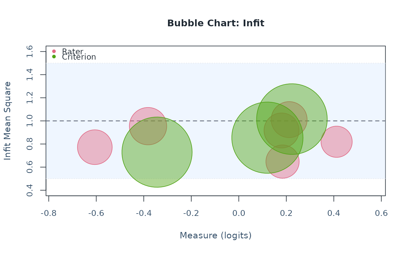# Above the review band: more response variation than expected; below: less
# By default, larger bubbles indicate greater precision, not greater misfit

# Optional: compare Infit (horizontal) and Outfit (vertical) directly
plot_bubble(fit, diagnostics = diagnostics, view = "infit_outfit")

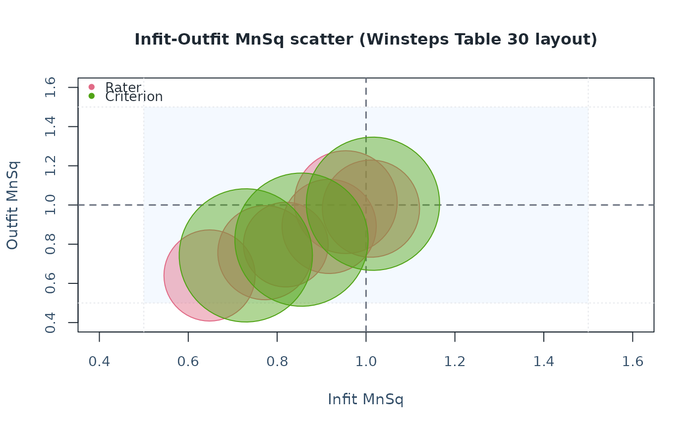# Here bubble size represents observation count; bands are review aids
# }