Plot per-rater severity ranking with confidence interval whiskers

Ranks the levels of a chosen rater facet by estimated severity and draws each level as a horizontal CI whisker around the point estimate. Optional descriptive bands mark absolute distances of 0.5 and 1.0 logit from zero; they are display aids, not calibration rules.

Usage

plot_rater_severity_profile(
  fit,
  diagnostics = NULL,
  facet = "Rater",
  ci_level = 0.95,
  show_bands = TRUE,
  preset = c("standard", "publication", "compact", "monochrome"),
  draw = TRUE
)

Arguments

fit: An mfrm_fit from fit_mfrm().
diagnostics: Optional diagnose_mfrm() output. When omitted, diagnose_mfrm(fit, residual_pca = "none") is run internally.
facet: Facet name to plot (default "Rater"). Any non-Person facet name is accepted.
ci_level: Confidence level used for the whiskers (default 0.95). Bounds use +/- z * ModelSE.
show_bands: Logical. When TRUE (default) draw shaded +/-0.5 and +/-1.0 logit guide bands and describe them in the subtitle and legend. Set to FALSE to omit both bands and their labels.
preset: Visual preset.
draw: If TRUE, draw with base graphics.

Value

An mfrm_plot_data object. Its data$data table contains columns Level, Estimate, SE, CI_Lower, CI_Upper, and Band. The enclosing data list retains the facet, confidence level and plot annotations; keep these with the table when reporting the results. Fit readiness and interpretation notes are retained; restricted fits are labeled REVIEW ONLY in the title.

Interpreting output

Zero is the sum-to-zero reference for the default centered facet; describe any different constraints or anchors used in the fit. With the default negative facet orientation, higher estimates mean stricter scoring. The optional bands and the legacy Band labels (gentle, moderate, strict) describe absolute magnitude, not the sign of severity, operational interchangeability, or a need for training. Pairwise claims require the uncertainty of the contrast; check the SE basis in the supplied diagnostics.

Session plot defaults

Set options(mfrmr.plot_preset = "publication") to choose a session default for plotting functions that expose the common preset argument. The supported values are "standard", "publication", "compact" and "monochrome". Precedence is an explicit call argument, then the session option, then "standard". For example, preset = "standard" overrides a session set to "monochrome". Explicit preset = NULL retains the earlier package-default behavior; it does not read the session option. Invalid session values cause an error only when that option is needed.

The category-curve, data-quality, fit-review, connectivity and network routes of plot() for report bundles use the same option through .... Plots without a common preset argument, including extended-model plots with their own palette controls, keep their own settings. This option selects a preset, not a universal theme or a guarantee that all renderers implement every appearance control identically.

New plot payloads retain the resolved preset for supported saved-data rendering. Converting an existing payload with as_ggplot() uses its saved appearance, even after the session option changes. A call that creates a new plot from a fit or statistical result uses the current default. For a reproducible script, supply preset explicitly or set the option in that script. Saving only the fitted model does not save a session option. No global ggplot theme is changed.

Restore previous settings with old <- options(mfrmr.plot_preset = "monochrome") followed by options(old). Use options(mfrmr.plot_preset = NULL) to remove the option. The preset changes appearance, not estimates, confidence levels or diagnostic thresholds.

Examples

# \donttest{
# Load the package and example ratings
library(mfrmr)
toy <- load_mfrmr_data("example_operational")

# Fit the model
fit <- fit_mfrm(
  data = toy,
  person = "Person",
  facets = c("Rater", "Criterion"),
  score = "Score",
  method = "MML",
  model = "RSM"
)

# Compute diagnostics once for the following checks
diagnostics <- diagnose_mfrm(fit)

# Compare signed severity estimates and their intervals
severity <- plot_rater_severity_profile(
  fit, diagnostics = diagnostics, show_bands = FALSE
)

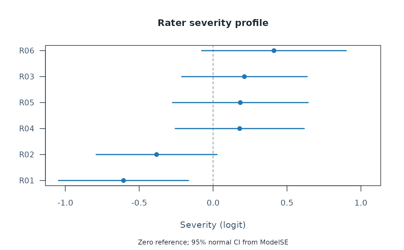severity$data$data[, c("Level", "Estimate", "SE", "CI_Lower", "CI_Upper")]
#>   Level   Estimate        SE    CI_Lower    CI_Upper
#> 1   R01 -0.6059776 0.2243521 -1.04569977 -0.16625550
#> 2   R02 -0.3820356 0.2085513 -0.79078871  0.02671748
#> 3   R04  0.1799462 0.2226570 -0.25645356  0.61634590
#> 4   R05  0.1842365 0.2341852 -0.27475809  0.64323116
#> 5   R03  0.2120388 0.2165999 -0.21248930  0.63656689
#> 6   R06  0.4117917 0.2494894 -0.07719839  0.90078189
# Higher estimates mean stricter ratings with this example's default orientation
# The optional magnitude bands are omitted from this first comparison
# }