Hierarchical grouping of external features

Build an agglomerative hierarchy from weighted Gower dissimilarities, cut it into a chosen number of groups, and inspect the retained dendrogram.

Usage

mfrm_cluster_hierarchical(
  x,
  k,
  weights = NULL,
  missing = c("error", "omit"),
  linkage = c("average", "complete")
)

# S3 method for class 'mfrm_hierarchical_clusters'
plot(
  x,
  type = c("dendrogram", "silhouette", "profile"),
  feature = NULL,
  labels = NULL,
  draw = TRUE,
  preset = "standard",
  ...
)

Arguments

x: For clustering, a table reviewed with mfrm_features(). For plotting, an mfrm_hierarchical_clusters result.
k: Number of groups, an integer from 2 to one less than the number of included entities, and no greater than their number of distinct profiles. The number is chosen by the user, not optimized automatically.
weights: Optional named, strictly positive finite numeric vector with one weight per selected feature. Defaults to equal weights. Names, not vector order, identify features. Remove a feature to exclude it.
missing: Either "error" (default) or "omit". The latter excludes incomplete entities explicitly, retaining their IDs, reasons, and missing group membership in the result. No values are imputed.
linkage: "average" (default, UPGMA) or "complete". Average linkage uses the mean dissimilarity over all cross-group pairs; complete linkage uses their maximum. Neither is selected automatically from the data.
type: "dendrogram" (default), "silhouette", or "profile".
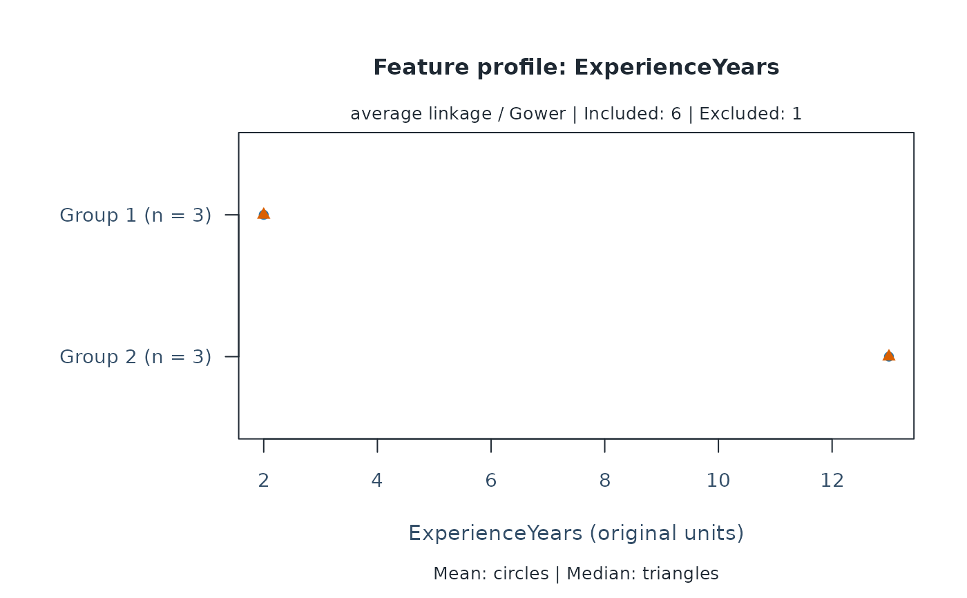
feature: A single selected feature name, required for type = "profile". Numeric features show means and medians in their original units; categorical features show within-group proportions in the original level order (including unused factor levels).
labels: Whether to display entity IDs on dendrograms and silhouettes. The default labels at most 50 included entities. Hiding labels does not remove entities. Profile plots always label groups and levels.
draw: Draw the plot when TRUE; FALSE only returns plotted values.
preset: Plot style: "standard", "publication", "compact", or "monochrome".
...: Reserved for future use; additional arguments are rejected.

Value

An mfrm_hierarchical_clusters object inheriting from mfrm_clusters. It retains the hclust object in tree, ID-aligned membership (ID, Cluster, Silhouette), cluster_summary, profiles, feature_data, and settings including the linkage. Hierarchical clustering does not select medoids; medoids is NULL and membership has no Medoid column. summary() returns the size/silhouette table. plot() invisibly returns mfrm_plot_data; dendrogram data include the tree, leaf order, memberships, group count, and excluded IDs.

Details

Uses stats::hclust() followed by stats::cutree() at the requested k. Feature types, scaling, weights, missingness handling, silhouette definition, and the 5,000-included-entity limit follow mfrm_cluster_pam(). No distance transformation or automatic sampling is performed. This limit is not a memory or speed guarantee.

Only average and complete linkage are supported. Ward's minimum-variance criterion requires an appropriate Euclidean geometry; this mixed-feature Gower interface does not define a Euclidean conversion or a Ward analysis. Clustering MFRM bias estimates is a separate methodological question from grouping the external attributes accepted here. Measurement uncertainty is not propagated.

The tree is fitted independently of PAM. Its merge heights describe the selected linkage on Gower dissimilarities, not significance or branch support. Tied distances can produce alternative hierarchies and input order can affect their resolution. A cut at k uses merge order even when heights tie, so a horizontal height threshold need not uniquely identify that cut.

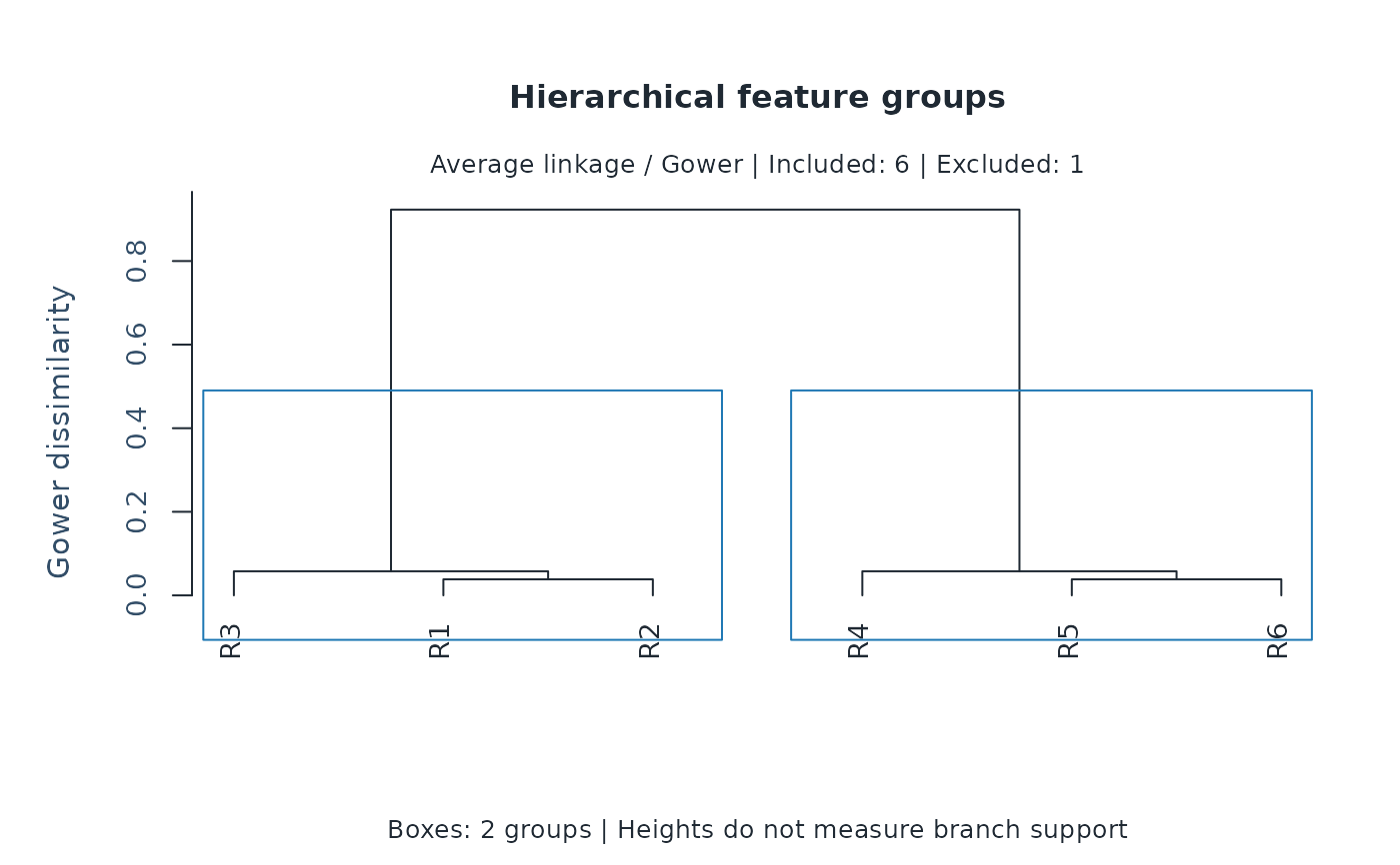
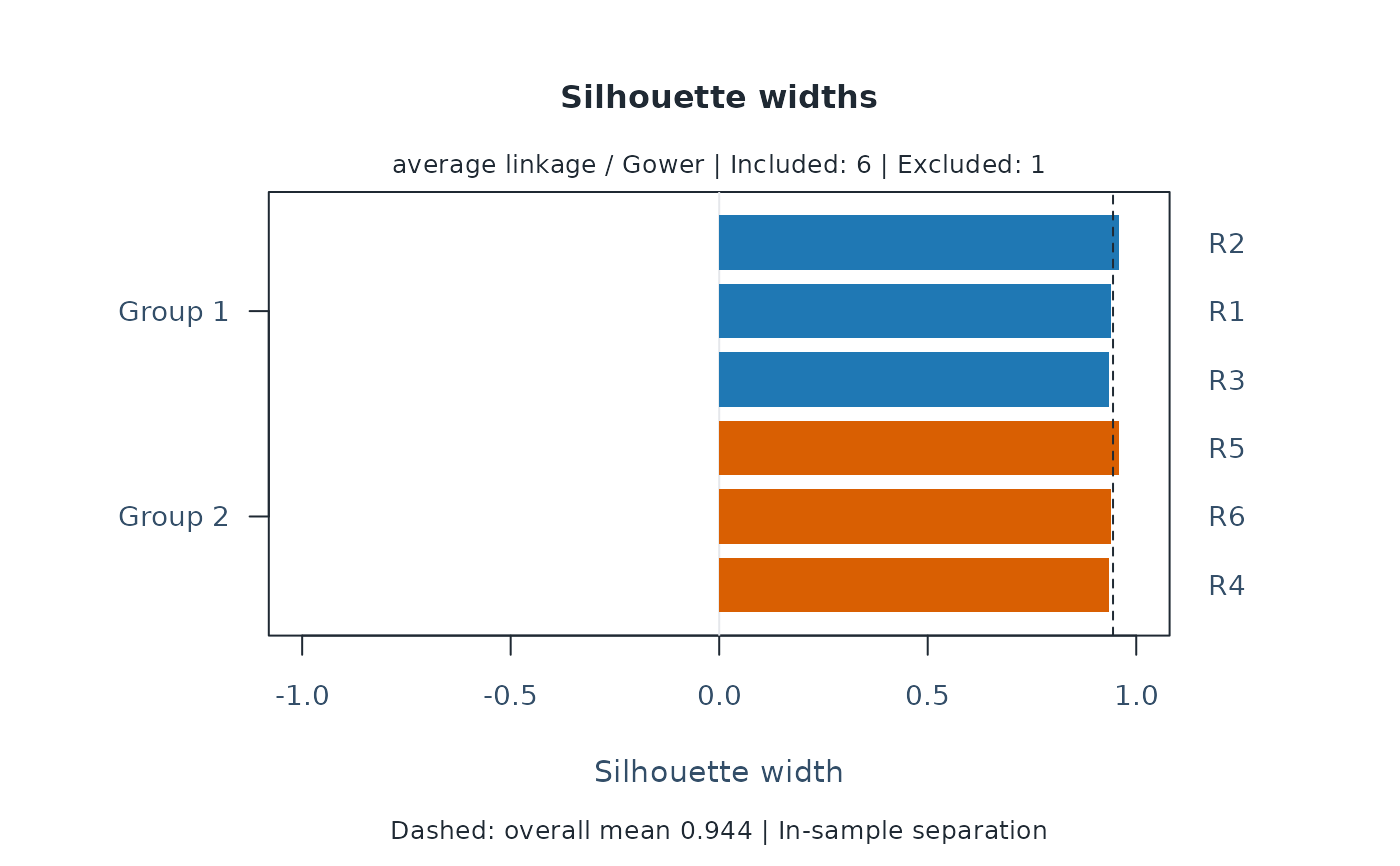
The default plot draws this stored tree, with boxes marking the stored k groups. Labels are shown for at most 50 included entities by default; hiding labels does not sample or remove entities. Excluded entities have no leaves but remain in the result and plot data. Silhouette and feature-profile views reuse plot.mfrm_clusters(). Plots do not refit or choose groups. as_ggplot() converts the stored dendrogram without refitting. The default and component = "tree" retain the full tree and group boxes. Leaf order, heights, label settings and excluded IDs are preserved. Dashed boxes differ from the solid tree branches even in monochrome. Box widths and physical text sizes can differ from base graphics. Tied heights retain the merge-order partition; boxes do not imply a unique horizontal height cut. Use ggplot2::labs(title = NULL, subtitle = NULL, caption = NULL) to remove headings and annotations, and plot_data() to inspect the retained source evidence. Silhouette/profile conversions use the same dedicated summary renderers as plot.mfrm_clusters().

Use mfrm_cluster_compare() to compare this partition with PAM or another linkage on the same data. For multiple imputations, use mfrm_cluster_imputed(..., method = "hierarchical", linkage = "average"). Each completion retains its own tree; no pooled tree or branch support is estimated. See vignette("mfrmr-external-features", package = "mfrmr").

Session plot defaults

Set options(mfrmr.plot_preset = "publication") to choose a session default for plotting functions that expose the common preset argument. The supported values are "standard", "publication", "compact" and "monochrome". Precedence is an explicit call argument, then the session option, then "standard". For example, preset = "standard" overrides a session set to "monochrome". Explicit preset = NULL retains the earlier package-default behavior; it does not read the session option. Invalid session values cause an error only when that option is needed.

The category-curve, data-quality, fit-review, connectivity and network routes of plot() for report bundles use the same option through .... Plots without a common preset argument, including extended-model plots with their own palette controls, keep their own settings. This option selects a preset, not a universal theme or a guarantee that all renderers implement every appearance control identically.

New plot payloads retain the resolved preset for supported saved-data rendering. Converting an existing payload with as_ggplot() uses its saved appearance, even after the session option changes. A call that creates a new plot from a fit or statistical result uses the current default. For a reproducible script, supply preset explicitly or set the option in that script. Saving only the fitted model does not save a session option. No global ggplot theme is changed.

Restore previous settings with old <- options(mfrmr.plot_preset = "monochrome") followed by options(old). Use options(mfrmr.plot_preset = NULL) to remove the option. The preset changes appearance, not estimates, confidence levels or diagnostic thresholds.

References

Murtagh, F. and Legendre, P. (2014). Ward's Hierarchical Agglomerative Clustering Method: Which Algorithms Implement Ward's Criterion? Journal of Classification, 31, 274–295. doi:10.1007/s00357-014-9161-z .

Examples

if (requireNamespace("cluster", quietly = TRUE)) {
  # Fictional rater backgrounds; R7 has unrecorded experience.
  raters <- data.frame(Rater = paste0("R", 1:7),
    ExperienceYears = c(1, 2, 3, 12, 13, 14, NA),
    Specialty = factor(c(rep("Language", 3), rep("Science", 4))))
  features <- mfrm_features(raters, "Rater", c("ExperienceYears", "Specialty"))
  hierarchy <- mfrm_cluster_hierarchical(features, k = 2, missing = "omit")
  plot(hierarchy)
  plot(hierarchy, type = "silhouette")
  plot(hierarchy, type = "profile", feature = "ExperienceYears")
  comparison <- mfrm_cluster_compare(list(
    PAM = mfrm_cluster_pam(features, k = 2, missing = "omit"),
    Average = hierarchy,
    Complete = mfrm_cluster_hierarchical(features, k = 2,
      linkage = "complete", missing = "omit")))
  comparison$analysis_summary
  summary(comparison)
}



#>     First   Second Partitions Included Pairs MeanChangedFraction
#> 1     PAM  Average          1        6    15                   0
#> 2     PAM Complete          1        6    15                   0
#> 3 Average Complete          1        6    15                   0
#>   MinChangedFraction MaxChangedFraction MeanAdjustedRand
#> 1                  0                  0                1
#> 2                  0                  0                1
#> 3                  0                  0                1