Review and plot portable fixed-calibration scores

These methods provide the first review surface for the result returned by score_mfrm_calibration(). print() gives a compact batch disposition, summary() exposes readable score and review tables, and plot() shows conditional score uncertainty or numerical review quantities without refitting a model.

Usage

# S3 method for class 'mfrm_calibration_score'
summary(object, digits = 3L, ...)

# S3 method for class 'mfrm_calibration_score'
print(x, ...)

# S3 method for class 'summary.mfrm_calibration_score'
print(x, ...)

# S3 method for class 'mfrm_calibration_score'
plot(
  x,
  type = c("interval", "precision", "edge_mass"),
  top_n = 40L,
  sort_by = c("estimate", "sd", "person"),
  label_review = TRUE,
  main = NULL,
  draw = TRUE,
  preset = c("standard", "publication", "compact", "monochrome"),
  ...
)

Arguments

object, x: An mfrm_calibration_score returned by score_mfrm_calibration().
digits: Number of decimal places in the summary.
...: Reserved for generic compatibility.
type: One of "interval", "precision", or "edge_mass".
top_n: Maximum number of scored Persons shown. Review rows are selected first when truncation is necessary. Use Inf to show all.
sort_by: Selection priority after review rows: absolute estimate, posterior SD, or Person identifier.
label_review: Whether review points are labelled in the precision and edge-mass views. Interval plots always label the displayed Persons.
main: Optional plot title.
draw: If TRUE, draw with base R graphics. The returned mfrm_plot_data is available invisibly in either case.
preset: Visual preset: "standard", "publication", "compact", or "monochrome".

Value

print() returns its input invisibly. summary() returns a summary.mfrm_calibration_score containing overview, estimates, review, row_review, settings, and notes. When adaptive integration was requested and scored rows exist, it also retains unrounded quadrature_review and a compact quadrature_overview. plot() returns an mfrm_plot_data with the selected plotting table, selection accounting, unplotted Person dispositions, interpretation guidance, and plotting settings.

Details

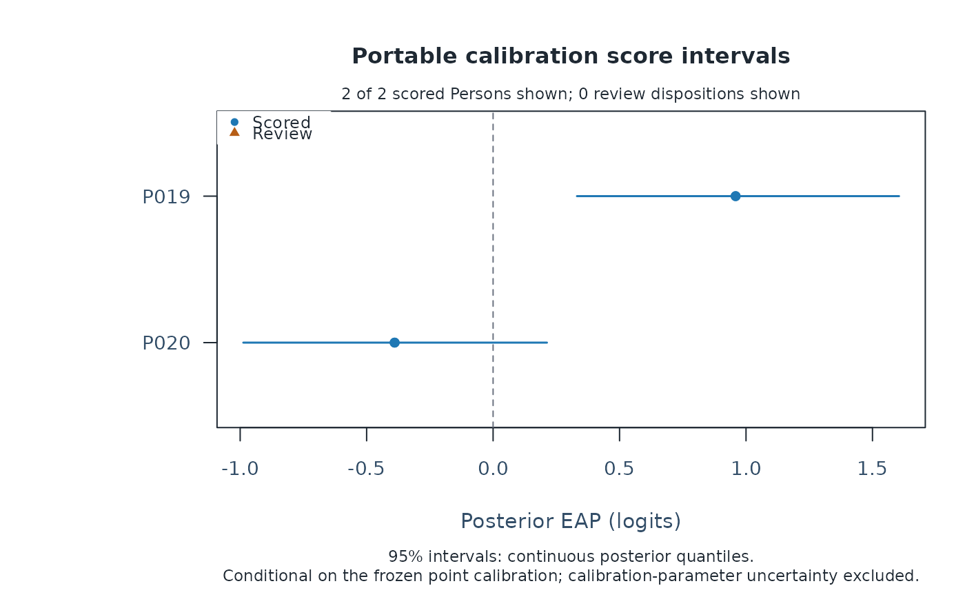
The default interval plot shows posterior EAP estimates and central intervals. type = "precision" plots the number of valid response rows against posterior SD. type = "edge_mass" compares posterior mass on the two outer quadrature nodes with the recorded review threshold. Review dispositions are highlighted in every view.

These are score-batch review displays, not calibration-fit diagnostics. Posterior SDs and intervals are conditional on the frozen point calibration and the actual scoring prior. They exclude calibration-parameter uncertainty. For GPCM or an explicitly supplied scoring prior, summaries and plot data retain both original and actual prior values without rounding, the per-Person integration checks, and (for GPCM) the source decision recorded at extraction. These records describe conditional scoring, not a new evaluation of the training fit or the suitability of its population for another cohort. summary(x)$settings$score_integration_review compares the reported EAP/SD with higher-order adaptive references. The separate quadrature_review compares adaptive and fixed grids; for an adaptive scorer, that fixed grid did not produce the reported scores. Printing distinguishes the two checks. Persons with no valid responses have no score coordinate and are retained in summary(x)$review and in the plot payload's unplotted_dispositions component.

The summary object retains every returned score and review disposition. Its estimates table preserves the available estimate and uncertainty basis columns, calibration identifiers, scoring algorithm and requested interval level when extracted or written to CSV. The interval level is not rounded. Older score results recover these fields from their recorded settings when re-summarized. Saved grid-based intervals retain their original endpoints; printed results and interval plots explain that their posterior mass can differ from the requested level. Its print method shows at most ten rows from each table so routine console output stays compact. Base and ggplot2 renderers distinguish scored and review states by shape as well as colour.

Session plot defaults

Set options(mfrmr.plot_preset = "publication") to choose a session default for plotting functions that expose the common preset argument. The supported values are "standard", "publication", "compact" and "monochrome". Precedence is an explicit call argument, then the session option, then "standard". For example, preset = "standard" overrides a session set to "monochrome". Explicit preset = NULL retains the earlier package-default behavior; it does not read the session option. Invalid session values cause an error only when that option is needed.

The category-curve, data-quality, fit-review, connectivity and network routes of plot() for report bundles use the same option through .... Plots without a common preset argument, including extended-model plots with their own palette controls, keep their own settings. This option selects a preset, not a universal theme or a guarantee that all renderers implement every appearance control identically.

New plot payloads retain the resolved preset for supported saved-data rendering. Converting an existing payload with as_ggplot() uses its saved appearance, even after the session option changes. A call that creates a new plot from a fit or statistical result uses the current default. For a reproducible script, supply preset explicitly or set the option in that script. Saving only the fitted model does not save a session option. No global ggplot theme is changed.

Restore previous settings with old <- options(mfrmr.plot_preset = "monochrome") followed by options(old). Use options(mfrmr.plot_preset = NULL) to remove the option. The preset changes appearance, not estimates, confidence levels or diagnostic thresholds.

Examples

# \donttest{
dat <- load_mfrmr_data("example_core")
ids <- unique(dat$Person)
training <- dat[dat$Person %in% ids[1:18], , drop = FALSE]
fit <- fit_mfrm(
  training, "Person", c("Rater", "Criterion"), "Score",
  model = "RSM", method = "MML", quad_points = 5, maxit = 20
)
q_review <- mml_quadrature_sensitivity(
  fit, training, quad_points = c(5, 7), theta_points = 41
)
fit <- q_review$fits$q7
calibration <- freeze_mfrm_calibration(
  validate_mfrm_calibration(extract_mfrm_calibration(
    fit, quadrature_review = q_review
  ))
)
new_rows <- dat[dat$Person %in% ids[19:20], , drop = FALSE]
scores <- score_mfrm_calibration(calibration, new_rows)
summary(scores)
#> mfrmr Portable Calibration Score Summary
#>   Calibration: mfrmr-calibration-v1:rsm:mml:20261002045420509003
#>   Model / estimator: RSM / MML
#>   Persons: 2 scored (0 requiring review); 0 not scored
#> 
#> Posterior estimates (2 of 2)
#>   P019: estimate 0.959, SD 0.328, interval [0.331, 1.605], scored
#>   P020: estimate -0.389, SD 0.311, interval [-0.988, 0.213], scored
#> 
#> Response-row disposition
#>   32 input; 32 scored; 0 omitted; 0 refused; missing-response policy: error
#> 
#> Interval interpretation
#>   95% intervals: continuous posterior quantiles.
#>   Posterior SDs and intervals are conditional on the frozen point calibration
#>   and exclude calibration-parameter uncertainty.
plot(scores, type = "interval")

plot(scores, type = "edge_mass", draw = FALSE)
# }