
Plot exploratory groups and imputation sensitivity
Source:R/api-plotting-clusters.R
plot.mfrm_clusters.RdInspect within-sample separation, individual feature profiles, or pairwise co-membership across imputations using existing clustering results.
Arguments
- x
An object returned by
mfrm_cluster_pam(),mfrm_cluster_kmeans()ormfrm_cluster_imputed(), as appropriate.- type
For a single partition,
"silhouette"or"profile".- feature
A single selected feature name, required for
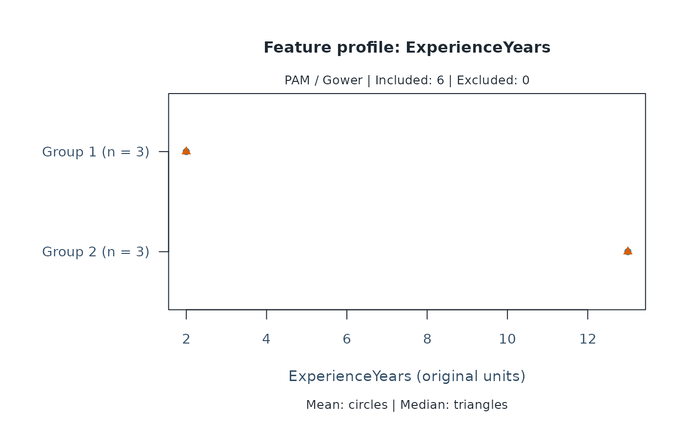
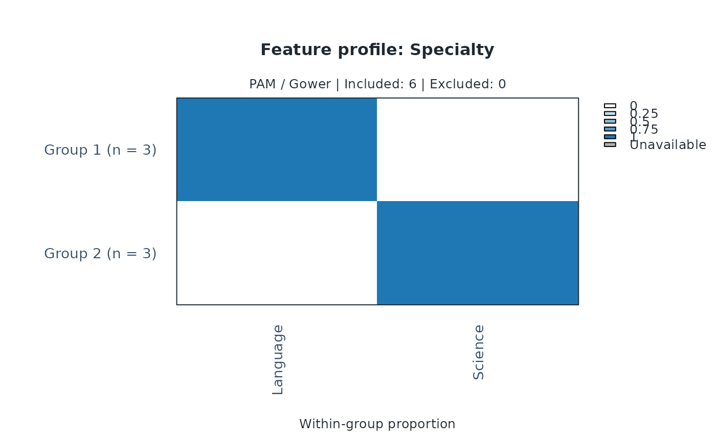
type = "profile". Numeric features show means and medians in their original units; categorical features show within-group proportions in the original level order (including unused factor levels).- labels
Whether to display entity IDs on silhouettes or heatmaps. The default displays them for at most 50 entities. No entities are sampled when labels are hidden. Profile plots always label groups and levels.
- draw
Draw the plot when
TRUE;FALSEonly returns plotted values.- preset
Plot style:
"standard","publication","compact", or"monochrome".- ...
Reserved for future use; additional arguments are rejected.
- ids
For imputation heatmaps, an optional character vector of distinct entity IDs in the desired display order. Selection affects only the view, not clustering or the denominator. By default all IDs appear in input order.
Value
Invisibly, an mfrm_plot_data object. Its data contains the plotted
table or matrix, title, subtitle, legend, and excluded IDs. Heatmaps also
retain the displayed IDs and the number of imputations. Use plot_data()
to extract this payload for custom graphics.
as_ggplot() converts imputation co-membership heatmaps using the saved
matrix, ID order, label choice, colours and imputation count. The default
and component = "matrix" retain the complete view and its fixed
zero-to-one scale. Unavailable cells have both grey fill and crosses,
distinguishing them from zero even in monochrome. Metadata, including
excluded IDs, remain available with plot_data(). No values are
recomputed or renormalized when IDs are selected. Use
ggplot2::labs(title = NULL, subtitle = NULL, caption = NULL) to hide
annotations while retaining the source data.
Silhouette conversion retains negative widths, saved order and the overall
mean reference, with group labels independent of colour. Numeric profiles
retain original-unit means/medians and counts; circles and triangles are
offset vertically to show coincident values without adding intervals.
Categorical profiles retain the original category order, unused levels,
group counts and a fixed zero-to-one proportion scale. Default and
component = "table" preserve the complete selected view; categorical
profiles also accept component = "matrix". These conversions do not
recluster, select groups, or estimate uncertainty.
Details
No model or clustering is refitted. Silhouette widths describe separation in the fitted sample, not stability or probabilities. The dashed line is the overall mean silhouette; excluded entities have no silhouette.
Feature profiles describe one partition; numeric summaries have no confidence
intervals. For an imputed result, inspect a completion with
plot(x$analyses[[1]], type = "profile", feature = "ExperienceYears").
Cluster numbers must not be averaged across imputations.
Imputation heatmaps show the fraction of all supplied imputations in which
each pair belongs to the same group, on a fixed zero-to-one scale. Grey cells
are unavailable pairs involving excluded entities, not zero co-membership.
These fractions describe sensitivity to imputations under fixed settings,
not membership probabilities, sampling stability, or a consensus partition.
Rows and columns follow input order or explicit ids; no hierarchical
clustering is performed. PAM is nonhierarchical and these plots do not
provide a dendrogram. Use mfrm_cluster_hierarchical() for a separate
hierarchical analysis and its dendrogram.
Session plot defaults
Set options(mfrmr.plot_preset = "publication") to choose a session default
for plotting functions that expose the common preset argument. The
supported values are "standard", "publication", "compact" and
"monochrome". Precedence is an explicit call argument, then the session
option, then "standard". For example, preset = "standard" overrides
a session set to "monochrome". Explicit preset = NULL retains the
earlier package-default behavior; it does not read the session option.
Invalid session values cause an error only when that option is needed.
The category-curve, data-quality, fit-review, connectivity and network
routes of plot() for report bundles use the same option through ....
Plots without a common preset argument, including extended-model plots
with their own palette controls, keep their own settings. This option
selects a preset, not a universal theme or a guarantee that all renderers
implement every appearance control identically.
New plot payloads retain the resolved preset for supported saved-data
rendering. Converting an existing payload with as_ggplot() uses its saved
appearance, even after the session option changes. A call that creates a
new plot from a fit or statistical result uses the current default.
For a reproducible script, supply preset explicitly or set the option in
that script. Saving only the fitted model does not save a session option.
No global ggplot theme is changed.
Restore previous settings with old <- options(mfrmr.plot_preset = "monochrome") followed by options(old). Use
options(mfrmr.plot_preset = NULL) to remove the option. The preset changes
appearance, not estimates, confidence levels or diagnostic thresholds.
Set options(mfrmr.plot_preset = "publication") to choose a session default
for plotting functions that expose the common preset argument. The
supported values are "standard", "publication", "compact" and
"monochrome". Precedence is an explicit call argument, then the session
option, then "standard". For example, preset = "standard" overrides
a session set to "monochrome". Explicit preset = NULL retains the
earlier package-default behavior; it does not read the session option.
Invalid session values cause an error only when that option is needed.
The category-curve, data-quality, fit-review, connectivity and network
routes of plot() for report bundles use the same option through ....
Plots without a common preset argument, including extended-model plots
with their own palette controls, keep their own settings. This option
selects a preset, not a universal theme or a guarantee that all renderers
implement every appearance control identically.
New plot payloads retain the resolved preset for supported saved-data
rendering. Converting an existing payload with as_ggplot() uses its saved
appearance, even after the session option changes. A call that creates a
new plot from a fit or statistical result uses the current default.
For a reproducible script, supply preset explicitly or set the option in
that script. Saving only the fitted model does not save a session option.
No global ggplot theme is changed.
Restore previous settings with old <- options(mfrmr.plot_preset = "monochrome") followed by options(old). Use
options(mfrmr.plot_preset = NULL) to remove the option. The preset changes
appearance, not estimates, confidence levels or diagnostic thresholds.
Examples
if (requireNamespace("cluster", quietly = TRUE)) {
raters <- data.frame(Rater = paste0("R", 1:6),
ExperienceYears = c(1, 2, 3, 12, 13, 14),
Specialty = factor(rep(c("Language", "Science"), each = 3)))
groups <- mfrm_cluster_pam(mfrm_features(raters, "Rater",
c("ExperienceYears", "Specialty")), k = 2)
plot(groups)
plot(groups, type = "profile", feature = "ExperienceYears")
plot(groups, type = "profile", feature = "Specialty")
values <- plot_data(plot(groups, draw = FALSE))
values$table
}
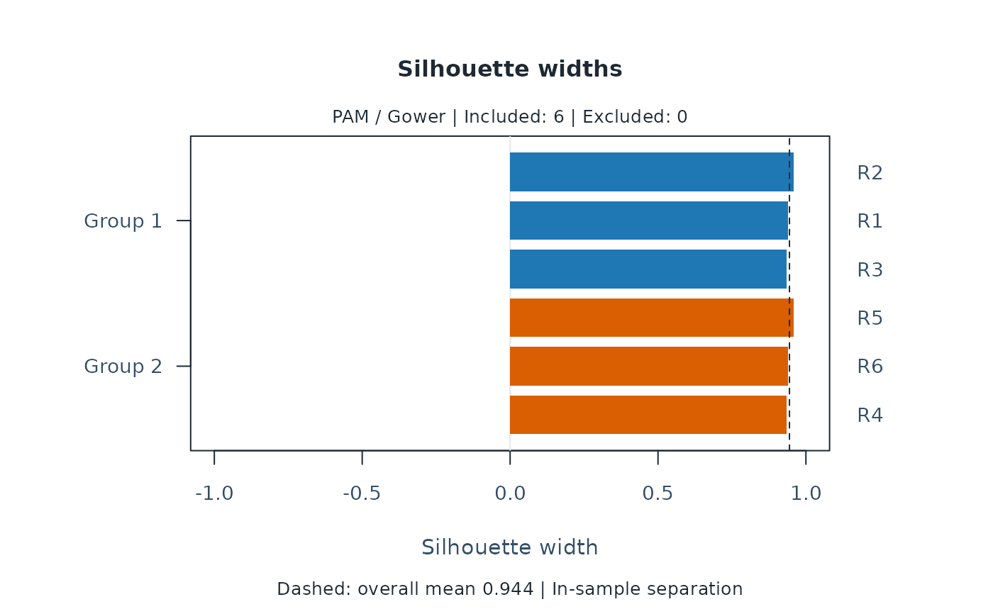
 #> ID Cluster Medoid Silhouette
#> 2 R2 1 TRUE 0.9583333
#> 1 R1 1 FALSE 0.9400000
#> 3 R3 1 FALSE 0.9347826
#> 5 R5 2 TRUE 0.9583333
#> 6 R6 2 FALSE 0.9400000
#> 4 R4 2 FALSE 0.9347826
#> ID Cluster Medoid Silhouette
#> 2 R2 1 TRUE 0.9583333
#> 1 R1 1 FALSE 0.9400000
#> 3 R3 1 FALSE 0.9347826
#> 5 R5 2 TRUE 0.9583333
#> 6 R6 2 FALSE 0.9400000
#> 4 R4 2 FALSE 0.9347826