Plot numeric feature PCA and optional exploratory groups

Review explained variation, original-feature coefficients or entity scores from a saved PCA without refitting it.

Usage

# S3 method for class 'mfrm_pca'
plot(
  x,
  type = c("scree", "scores", "loadings"),
  components = NULL,
  groups = NULL,
  labels = NULL,
  draw = TRUE,
  preset = "standard",
  ...
)

Arguments

x: A result from mfrm_pca().
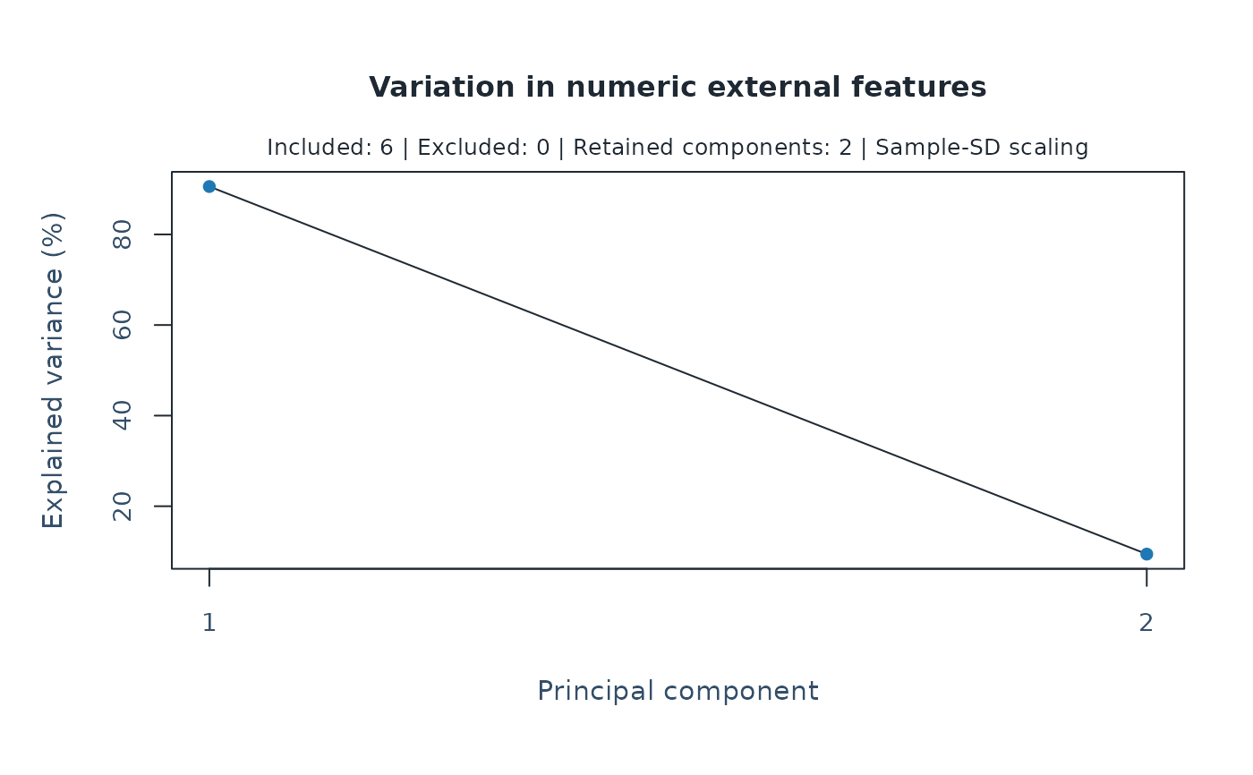
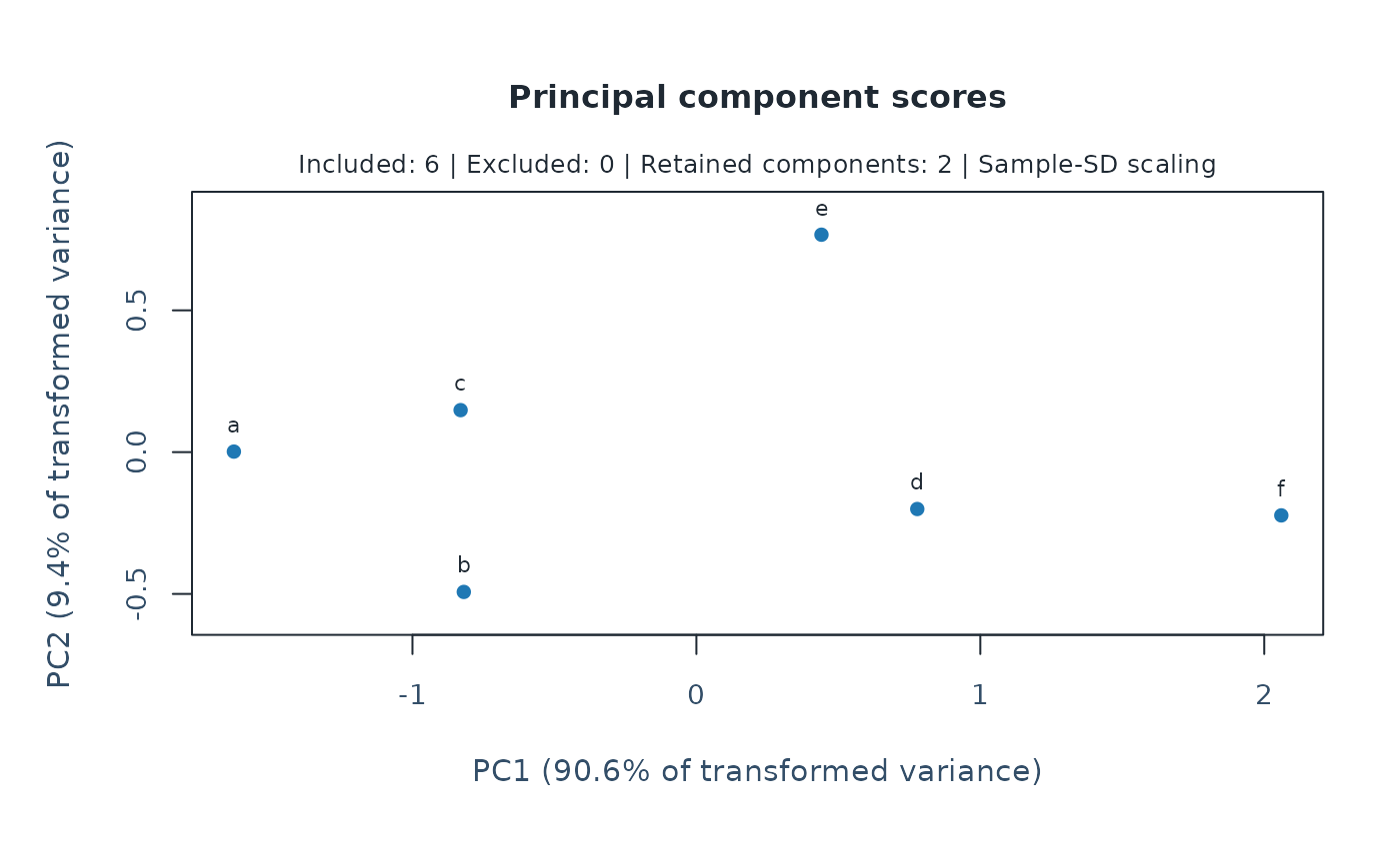
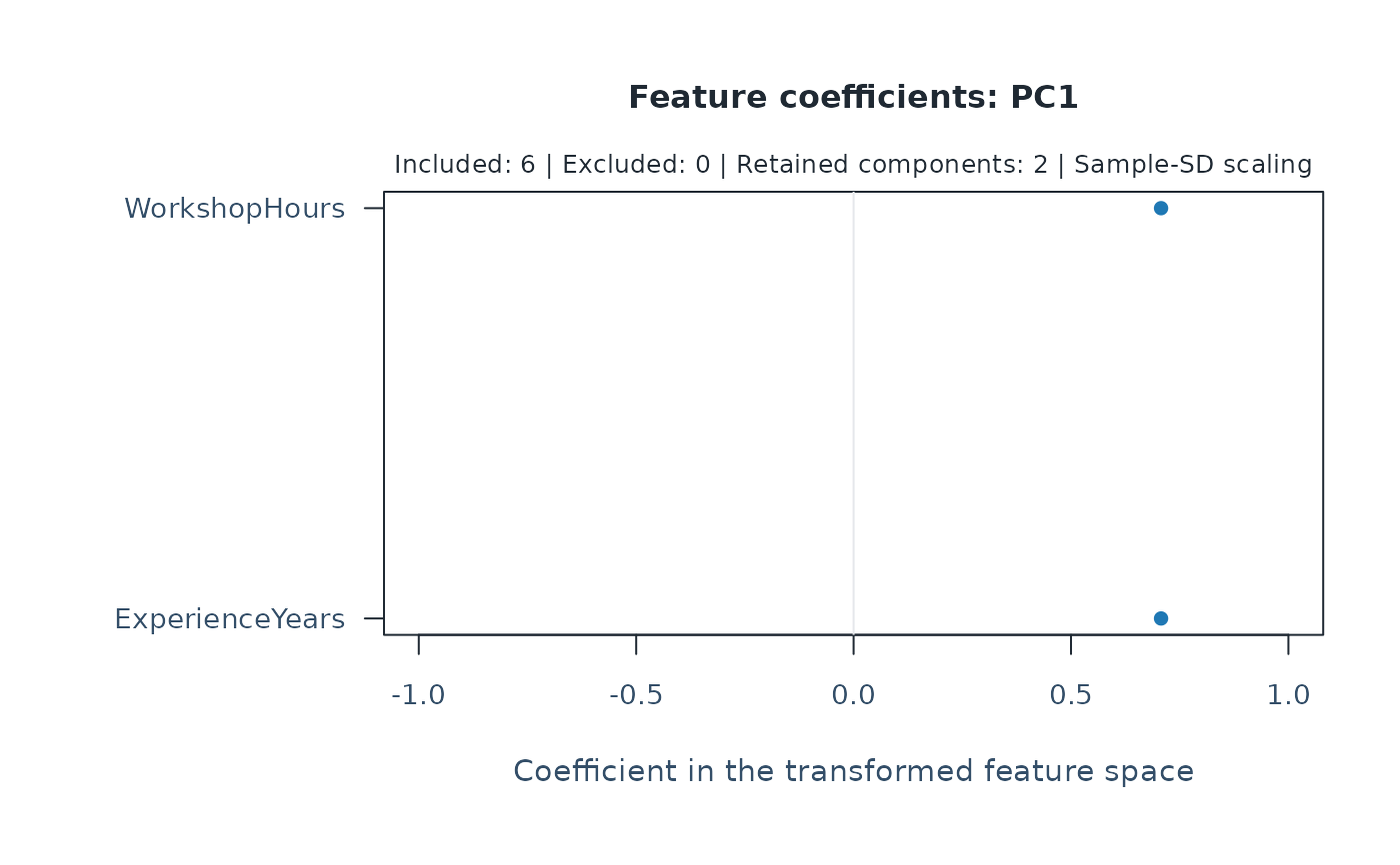
type: "scree" (default), "scores", or "loadings".
components: For scores, two distinct retained component numbers. For loadings, one retained component number. Defaults to c(1, 2) for scores and 1 for loadings. Unavailable axes cause an error.
groups: Optional mfrm_cluster_kmeans(), mfrm_cluster_pam() or mfrm_cluster_hierarchical() result used to color a scores plot. Its IDs, included entities and shared PCA features must match. Labels only annotate the view; they do not refit PCA or imply separation on every component. Groups use both colour and point shape, including monochrome output. Shapes repeat after six groups; inspect the ID-aligned table for crowded views.
labels: Whether to display entity IDs on silhouettes or heatmaps. The default displays them for at most 50 entities. No entities are sampled when labels are hidden. Profile plots always label groups and levels.
draw: Draw the plot when TRUE; FALSE only returns plotted values.
preset: Plot style: "standard", "publication", "compact", or "monochrome".
...: Reserved for future use; additional arguments are rejected.

Value

Invisibly, an mfrm_plot_data object with the exact plotted table, selected components, group colour/shape encoding, excluded IDs and axis meanings. Scree data retain the full variance table, including components not used for clustering. plot_data() extracts these values. as_ggplot() converts all three views using their saved axes and encodings; component = "table" retains the complete view. Excluded IDs and transformation metadata remain attached. Use ggplot2::labs(title = NULL, subtitle = NULL) to hide headings in the returned ggplot. Labels follow the saved labels setting; no entities are sampled when labels are hidden. Physical text and point sizes can differ between base graphics and ggplot. Converted scores use equal axis units and equal displayed spans to avoid a narrow panel when the selected components explain very different amounts of variation.

Details

Scores and loading signs are arbitrary. Loadings are eigenvector coefficients in the centered, weighted and optionally standardized space; they are not original-unit correlations. A two-component scores view omits other directions, so apparent overlap or separation is only a projection. No confidence region, group validity or rater-quality judgment is implied.

Session plot defaults

Set options(mfrmr.plot_preset = "publication") to choose a session default for plotting functions that expose the common preset argument. The supported values are "standard", "publication", "compact" and "monochrome". Precedence is an explicit call argument, then the session option, then "standard". For example, preset = "standard" overrides a session set to "monochrome". Explicit preset = NULL retains the earlier package-default behavior; it does not read the session option. Invalid session values cause an error only when that option is needed.

The category-curve, data-quality, fit-review, connectivity and network routes of plot() for report bundles use the same option through .... Plots without a common preset argument, including extended-model plots with their own palette controls, keep their own settings. This option selects a preset, not a universal theme or a guarantee that all renderers implement every appearance control identically.

New plot payloads retain the resolved preset for supported saved-data rendering. Converting an existing payload with as_ggplot() uses its saved appearance, even after the session option changes. A call that creates a new plot from a fit or statistical result uses the current default. For a reproducible script, supply preset explicitly or set the option in that script. Saving only the fitted model does not save a session option. No global ggplot theme is changed.

Restore previous settings with old <- options(mfrmr.plot_preset = "monochrome") followed by options(old). Use options(mfrmr.plot_preset = NULL) to remove the option. The preset changes appearance, not estimates, confidence levels or diagnostic thresholds.

Examples

attributes <- data.frame(ID = letters[1:6],
  ExperienceYears = c(1, 2, 4, 8, 10, 12),
  WorkshopHours = c(8, 16, 12, 24, 16, 32))
result <- mfrm_pca(mfrm_features(attributes, "ID", names(attributes)[-1]))
plot(result)

plot(result, type = "scores")

plot(result, type = "loadings", components = 1)

plot_data(plot(result, type = "scores", draw = FALSE))$table
#>   ID        PC1          PC2 Cluster
#> 1  a -1.6289491  0.001871076      NA
#> 2  b -0.8191619 -0.492997833      NA
#> 3  c -0.8304076  0.148084532      NA
#> 4  d  0.7779212 -0.200570920      NA
#> 5  e  0.4405114  0.766675482      NA
#> 6  f  2.0600859 -0.223062336      NA