Compare Wright maps or category curves from two fitted models

Usage

plot_compare_mfrm(
  reference,
  comparison,
  type = c("wright", "ccc"),
  view = c("comparison", "difference"),
  labels = c("Reference", "Comparison"),
  curve_groups = NULL,
  panel = c("auto", "category", "group"),
  theta_range = c(-6, 6),
  theta_points = 241L,
  preset = c("standard", "publication", "compact", "monochrome"),
  show_title = TRUE,
  show_notes = TRUE,
  draw = TRUE
)

Arguments

reference, comparison: Two mfrm_fit objects. All signed differences are comparison minus reference, on the fitted coordinate scale.
type: "wright" for distributions/locations or "ccc" for category probabilities at the zero additive-facet reference profile.
view: "comparison" for paired displays or "difference" for matched location differences versus means, or probability differences.
labels: Two distinct, nonempty display labels, reference first.
curve_groups: Optional step-facet levels to compare. By default all groups are required in both fits. An RSM common scale is explicitly paired with each selected PCM/GPCM group. Non-RSM fits must share a step owner.
panel: CCC layout: "auto" uses category panels in monochrome or with more than five categories, otherwise "group". "category" always separates categories; "group" overlays categories within each group.
theta_range: Finite increasing length-two predictor range for CCCs.
theta_points: Integer number of grid points, at least two.
preset: Existing visual preset; monochrome uses shapes/line types as well as grey tones.
show_title, show_notes: Display title and explanatory subtitle. Notes and source readiness remain in the returned object.
draw: Draw with the optional ggplot2 renderer. FALSE returns data without requiring ggplot2. Use as_ggplot() to customize/export a view.

Value

An mfrm_plot_data object. data$locations and data$differences describe Wright coordinates and matches; data$probabilities, data$differences and data$summary describe CCCs. Both types return group_selection, category_labels, basis, scale_contracts, fit_readiness, notes and display settings. source_plots preserves the native draw-free payloads and their exclusions/interpretation metadata.

Details

This is a descriptive paired-model display, not an information-criterion comparison or an external-software importer. Recorded centering, anchors, orientation, category coding, estimator method and coordinate basis must agree. These checks do not establish scale equivalence: no origin or unit transformation is estimated, and no observations or model parameters are refitted. Population SDs, full scale contracts and compared settings are returned for inspection. Different data/assignments can affect differences.

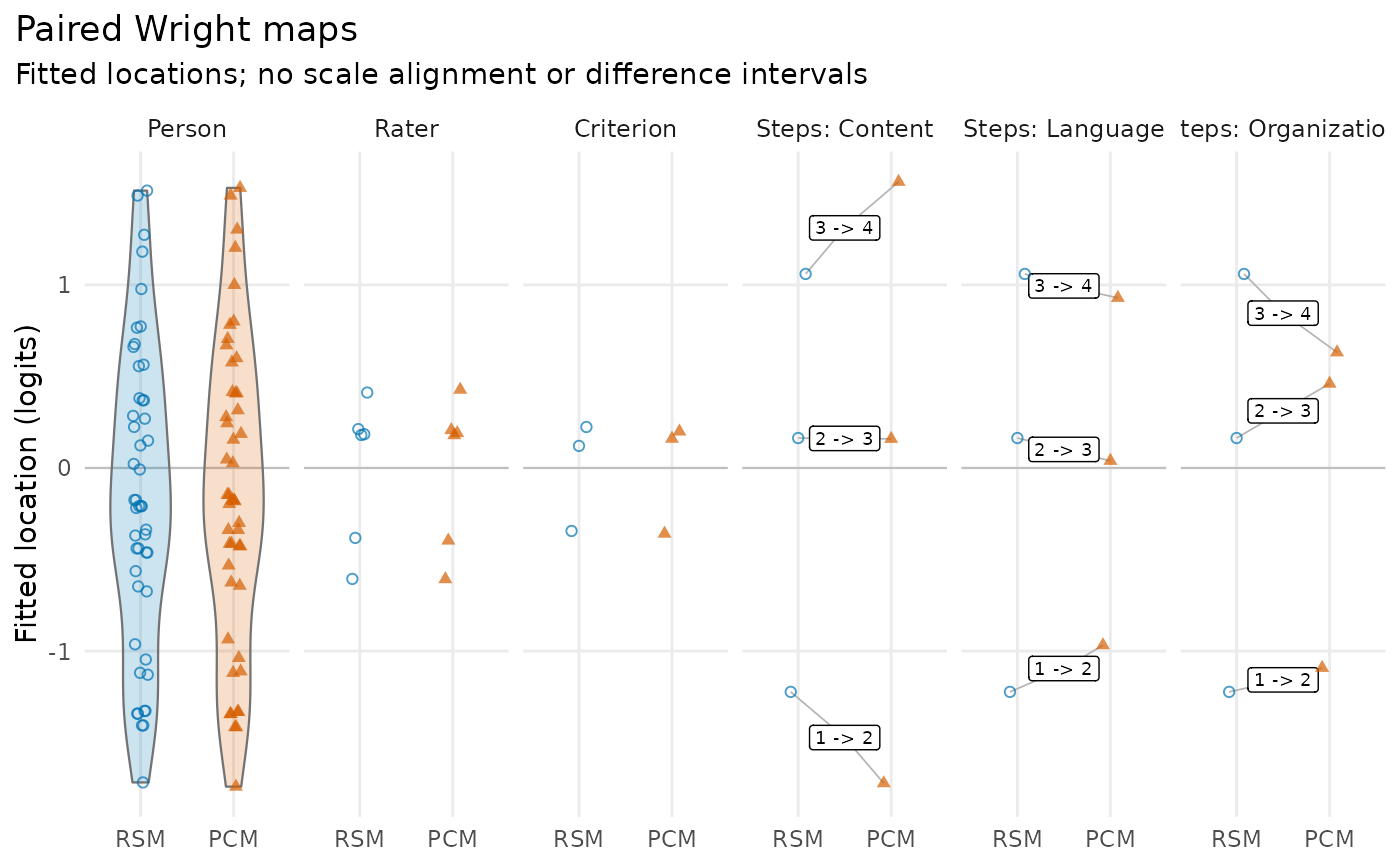
Wright maps use all source levels, with persons displayed as violins only when at least two distinct eligible estimates exist; otherwise points are used. Facet and step points are offset horizontally only. Step panels pair corresponding adjacent transitions; RSM steps are repeated as references across selected PCM/GPCM groups, not estimated separately. Excluded, non-finite, boundary-separated and unmatched levels remain in the tables. Differences are unavailable for those rows, never set to zero. No SE or CI for a difference is calculated. Person distributions are distributions of fitted point estimates, not posterior or population density estimates.

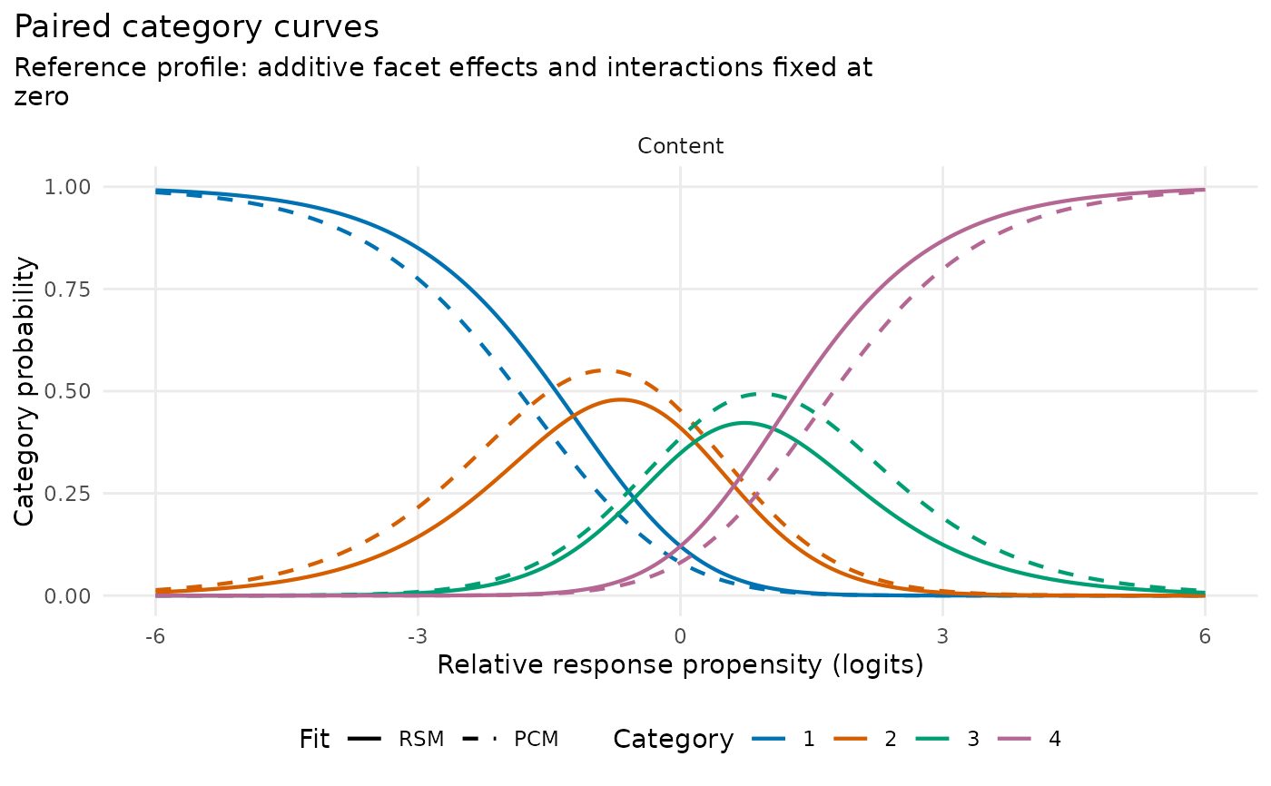
CCCs reuse plot.mfrm_fit() probabilities, retaining GPCM slopes. Additive facet effects and interactions are fixed at zero in both fits. Equal original category mappings and a common predictor grid are required. The maximum absolute probability difference is a grid diagnostic, with its signed value, category and grid location from the first maximizing row returned; it is not a continuous-domain supremum or a significance test. Use explicit group selection or a larger export when many panels are needed. Category retains the native internal code; OriginalCategory records the score label shown in the plot. ExpectedScoreDifference uses the native internal score coding, which need not equal the original score increments.

Session plot defaults

Set options(mfrmr.plot_preset = "publication") to choose a session default for plotting functions that expose the common preset argument. The supported values are "standard", "publication", "compact" and "monochrome". Precedence is an explicit call argument, then the session option, then "standard". For example, preset = "standard" overrides a session set to "monochrome". Explicit preset = NULL retains the earlier package-default behavior; it does not read the session option. Invalid session values cause an error only when that option is needed.

The category-curve, data-quality, fit-review, connectivity and network routes of plot() for report bundles use the same option through .... Plots without a common preset argument, including extended-model plots with their own palette controls, keep their own settings. This option selects a preset, not a universal theme or a guarantee that all renderers implement every appearance control identically.

New plot payloads retain the resolved preset for supported saved-data rendering. Converting an existing payload with as_ggplot() uses its saved appearance, even after the session option changes. A call that creates a new plot from a fit or statistical result uses the current default. For a reproducible script, supply preset explicitly or set the option in that script. Saving only the fitted model does not save a session option. No global ggplot theme is changed.

Restore previous settings with old <- options(mfrmr.plot_preset = "monochrome") followed by options(old). Use options(mfrmr.plot_preset = NULL) to remove the option. The preset changes appearance, not estimates, confidence levels or diagnostic thresholds.

Examples

# \donttest{
# Load one dataset for both models
library(mfrmr)
toy <- load_mfrmr_data("example_operational")

# RSM: shared category thresholds
fit_rsm <- fit_mfrm(
  data = toy,
  person = "Person",
  facets = c("Rater", "Criterion"),
  score = "Score",
  method = "MML",
  model = "RSM"
)

# PCM: separate category thresholds for each criterion
fit_pcm <- fit_mfrm(
  data = toy,
  person = "Person",
  facets = c("Rater", "Criterion"),
  score = "Score",
  method = "MML",
  model = "PCM",
  step_facet = "Criterion"
)

# Compare fitted locations; drawing requires the optional ggplot2 package
# If needed, install it once with install.packages("ggplot2")
if (requireNamespace("ggplot2", quietly = TRUE)) {
  plot_compare_mfrm(fit_rsm, fit_pcm, labels = c("RSM", "PCM"))

  # Run separately: compare score-category probabilities for one criterion
  plot_compare_mfrm(
    fit_rsm, fit_pcm,
    type = "ccc",
    curve_groups = "Content",
    labels = c("RSM", "PCM")
  )
}



# Plot data are available even without ggplot2
paired <- plot_compare_mfrm(fit_rsm, fit_pcm, draw = FALSE)
head(paired$data$differences)
#>     Kind  Facet Level Estimate_Reference SourceEstimate_Reference
#> 1 Person Person  P001         0.28429588               0.28429588
#> 2 Person Person  P002         0.66118004               0.66118004
#> 3 Person Person  P003         0.02177773               0.02177773
#> 4 Person Person  P004         0.22410785               0.22410785
#> 5 Person Person  P005        -0.17496065              -0.17496065
#> 6 Person Person  P006         0.67681003               0.67681003
#>   Status_Reference Estimate_Comparison SourceEstimate_Comparison
#> 1        available          0.27759201                0.27759201
#> 2        available          0.66997152                0.66997152
#> 3        available          0.04626811                0.04626811
#> 4        available          0.24404608                0.24404608
#> 5        available         -0.14689383               -0.14689383
#> 6        available          0.70466790                0.70466790
#>   Status_Comparison   Difference        Mean
#> 1         available -0.006703866  0.28094394
#> 2         available  0.008791479  0.66557578
#> 3         available  0.024490385  0.03402292
#> 4         available  0.019938230  0.23407696
#> 5         available  0.028066825 -0.16092724
#> 6         available  0.027857869  0.69073897
# Differences are PCM minus RSM; no difference SE or significance test is computed
# }