Plot a base-R QC dashboard

Usage

plot_qc_dashboard(
  fit,
  diagnostics = NULL,
  threshold_profile = "standard",
  thresholds = NULL,
  abs_z_min = 2,
  prob_max = 0.3,
  rater_facet = NULL,
  interrater_exact_warn = 0.5,
  interrater_corr_warn = 0.3,
  fixed_p_max = 0.05,
  random_p_max = 0.05,
  top_n = 20,
  draw = TRUE,
  preset = c("standard", "publication", "compact", "monochrome")
)

Arguments

fit: Output from fit_mfrm().
diagnostics: Optional output from diagnose_mfrm().
threshold_profile: Threshold profile name (strict, standard, lenient).
thresholds: Optional named threshold overrides.
abs_z_min: Absolute standardized-residual cutoff for unexpected panel.
prob_max: Maximum observed-category probability cutoff for unexpected panel.
rater_facet: Optional rater facet used in inter-rater panel.
interrater_exact_warn: Warning threshold for inter-rater exact agreement.
interrater_corr_warn: Warning threshold for inter-rater correlation.
fixed_p_max: Warning cutoff for fixed-effect facet chi-square p-values.
random_p_max: Warning cutoff for random-effect facet chi-square p-values.
top_n: Maximum elements displayed in displacement panel.
draw: If TRUE, draw with base graphics.
preset: Visual preset ("standard", "publication", "compact", or "monochrome").

Value

A plotting-data object of class mfrm_plot_data.

Details

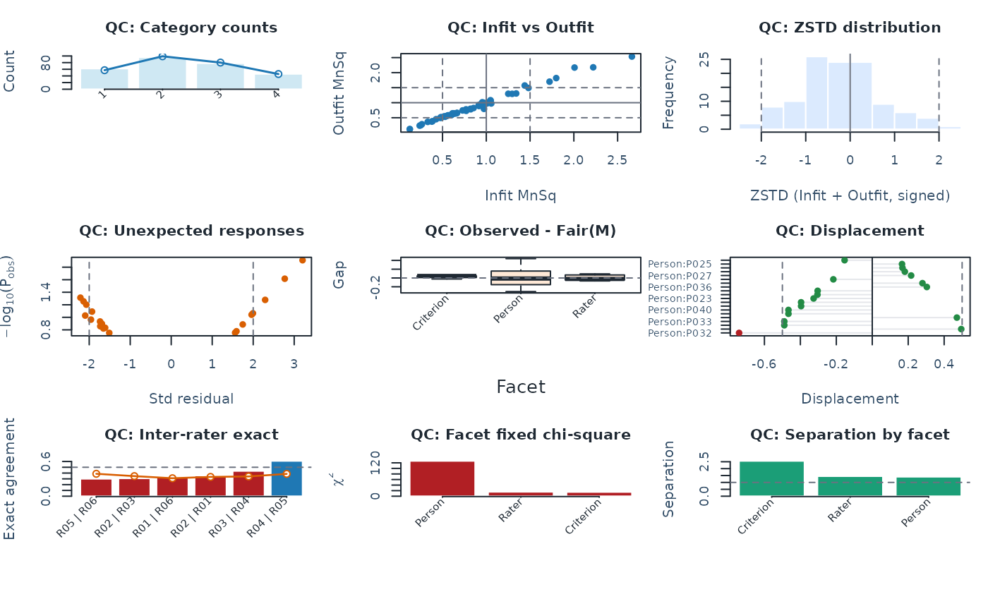
The dashboard draws nine QC panels in a 3\(\times\)3 grid:

Panel	What it shows	Key reference lines
1. Category counts	Observed (bars) vs model-expected counts (line)	–
2. Infit vs Outfit	Scatter of element MnSq values	heuristic 0.5, 1.0, 1.5 bands
3. \|ZSTD\| histogram	Distribution of absolute standardised residuals	\|ZSTD\| = 2
4. Unexpected responses	Standardised residual vs \(-\log_{10} P_{\mathrm{obs}}\)	`abs_z_min`, `prob_max`
5. Fair-average gaps	Boxplots of (Observed - FairM) per facet	zero line
6. Displacement	Top absolute displacement values	\(\pm 0.5\) logits
7. Inter-rater agreement	Exact agreement with expected overlay per pair	`interrater_exact_warn`
8. Fixed chi-square	Fixed-effect \(\chi^2\) per facet	`fixed_p_max`
9. Separation & Reliability	Bar chart of separation index per facet	–

threshold_profile controls warning overlays. Three built-in profiles are available: "strict", "standard" (default), and "lenient". Use thresholds to override any profile value with named entries.

For GPCM, the dashboard now reuses the residual-based diagnostics stack and marks the fair-average panel unavailable rather than silently reusing the Rasch-only compatibility calculation.

Plot types

This function draws a fixed 3\(\times\)3 panel grid (no plot_type argument). For individual panel control, use the dedicated helpers: plot_unexpected(), plot_fair_average(), plot_displacement(), plot_interrater_agreement(), plot_facets_chisq().

Interpreting output

Recommended panel order for fast review:

Category counts + Infit/Outfit (row 1): first-pass model screening. Category bars should roughly track the expected line; Infit/Outfit points are often reviewed against the heuristic 0.5–1.5 band.
Unexpected responses + Displacement (row 2): element-level outliers. Sparse points and small displacements are desirable.
Inter-rater + Chi-square (row 3): facet-level comparability. Read these as screening panels: higher agreement suggests stronger scoring consistency, and significant fixed chi-square indicates detectable facet spread under the current model.
Separation/Reliability (row 3): approximate screening precision. Higher separation indicates more statistically distinct strata under the current SE approximation.

Treat this dashboard as a screening layer; follow up with dedicated helpers (plot_unexpected(), plot_displacement(), plot_interrater_agreement(), plot_facets_chisq()) for detailed diagnosis.

Typical workflow

Fit and diagnose model.
Run plot_qc_dashboard() for one-page triage.
Drill into flagged panels using dedicated functions.

Session plot defaults

Set options(mfrmr.plot_preset = "publication") to choose a session default for plotting functions that expose the common preset argument. The supported values are "standard", "publication", "compact" and "monochrome". Precedence is an explicit call argument, then the session option, then "standard". For example, preset = "standard" overrides a session set to "monochrome". Explicit preset = NULL retains the earlier package-default behavior; it does not read the session option. Invalid session values cause an error only when that option is needed.

The category-curve, data-quality, fit-review, connectivity and network routes of plot() for report bundles use the same option through .... Plots without a common preset argument, including extended-model plots with their own palette controls, keep their own settings. This option selects a preset, not a universal theme or a guarantee that all renderers implement every appearance control identically.

New plot payloads retain the resolved preset for supported saved-data rendering. Converting an existing payload with as_ggplot() uses its saved appearance, even after the session option changes. A call that creates a new plot from a fit or statistical result uses the current default. For a reproducible script, supply preset explicitly or set the option in that script. Saving only the fitted model does not save a session option. No global ggplot theme is changed.

Restore previous settings with old <- options(mfrmr.plot_preset = "monochrome") followed by options(old). Use options(mfrmr.plot_preset = NULL) to remove the option. The preset changes appearance, not estimates, confidence levels or diagnostic thresholds.

Examples

# \donttest{
# Load the package and example ratings
library(mfrmr)
toy <- load_mfrmr_data("example_operational")

# Fit the model
fit <- fit_mfrm(
  data = toy,
  person = "Person",
  facets = c("Rater", "Criterion"),
  score = "Score",
  method = "MML",
  model = "RSM"
)

# Compute diagnostics once for the following checks
diagnostics <- diagnose_mfrm(fit)

# Read the interpretation status before reviewing the quality-control (QC) panels
review <- summary(diagnostics)
review$decision
#>               Interpretation FormalInference FitReadiness
#> 1 Ready for formal inference             Yes        ready
#>                                           Why
#> 1 All stored fit-readiness components passed.
#>                                                                                            NextAction
#> 1 Inspect `diagnostic_basis` before comparing legacy residual evidence with strict marginal evidence.

# Draw the dashboard and save its data
qc <- plot_qc_dashboard(fit, diagnostics = diagnostics)


# Inspect the counts behind the category panel
qc$data$category_stats[, c("Category", "Count", "ExpectedCount")]
#> # A tibble: 4 × 3
#>   Category Count ExpectedCount
#>      <int> <dbl>         <dbl>
#> 1        1    62          57.2
#> 2        2    96          99.0
#> 3        3    78          80.1
#> 4        4    46          45.6
# Use focused plots such as plot_marginal_fit(diagnostics) to investigate a panel
# }