Connect rating designs, network diagnostics and reports • mfrmr

Start with the decision: can these ratings support the comparison you need, what differs between raters, and what should change in the next assessment? Networks help at different stages. Their nodes and edges determine what they can say; a similar-looking diagram does not make two analyses equivalent.

Stage and question	Nodes / edges	Connect to
Before fitting: who is linked to whom?	Person/facet levels; planned or observed co-occurrence counts	`subset_connectivity_report(data = ...)` → `mfrm_network_analysis()` / `build_mfrm_network_review()` → collection/linking decisions
After reviewing the fit: which raters agree or score higher?	Raters; matched observed-score agreement or directional discrepancies	`interrater_agreement_table()` → `rater_network_analysis()` → examine MFRM severity and specified bias contrasts
Do criteria scored by the same rater co-move?	Rater × criterion profiles; observed-score correlations	`rater_halo_network_analysis()` → inspect within-/between-rater associations and substantive rubric explanations
What remains after the fitted model?	Facet levels; correlations of Person-level mean standardized residuals	`mfrm_residual_network()` → exploratory matrix/tree → a separately justified model or validation study
Which external profiles look similar?	One row per entity; declared feature distances	`mfrm_features()` → PCA/PAM/k-means/hierarchy → profiles and sensitivity review

The first graph does not establish model identification. The next two do not adjust scores for task difficulty or person ability. The residual route depends on the fitted model and aggregation. None is a causal network or proof of latent classes. Fixed criteria in a multivariate G-study are a vector of observed scores, not automatically either MFRM facets or latent dimensions.

Inspect the design before estimating a model

Start with the bundled observed ratings. facets = "Rater" deliberately shows only person-rater links; the full MFRM can still contain Criterion.

ratings <- load_mfrmr_data("example_operational")
if (requireNamespace("igraph", quietly = TRUE)) {
  observed <- mfrm_network_analysis(data = ratings, person = "Person",
    facets = "Rater", score = "Score")
  observed$summary
  head(observed$source_connectivity$row_usage)
}
#>   Row Included   Reason
#> 1   1     TRUE Included
#> 2   2     TRUE Included
#> 3   3     TRUE Included
#> 4   4     TRUE Included
#> 5   5     TRUE Included
#> 6   6     TRUE Included

Each retained row adds one co-observation to each selected pair of facet levels. Repeated rows therefore increase edge counts; they are not independent-person sample sizes. Missing scores do not create observed edges. Known levels in unscored rows remain as isolates. Supply a complete assignment roster to see planned links; levels absent from the supplied file cannot be invented.

The next example constructs a planned assignment, because changing an assignment is the object of this lesson. There are 48 persons and 12 raters in three panels, with two raters per person. One extra rating connects two panels; the third remains separate. It is an illustrative plan, not simulated evidence about estimator performance.

assignment <- do.call(rbind, lapply(1:48, function(i) {
  panel <- (i - 1L) %/% 16L
  local <- (i - 1L) %% 4L
  data.frame(Person = paste0("P", i),
    Rater = paste0("R", panel * 4L + c(local + 1L, (local + 1L) %% 4L + 1L)))
}))
linked_assignment <- rbind(assignment, data.frame(Person = "P16", Rater = "R5"))
if (requireNamespace("igraph", quietly = TRUE)) {
  before <- mfrm_network_analysis(data = assignment, person = "Person",
    facets = "Rater", basis = "planned")
  after <- mfrm_network_analysis(data = linked_assignment, person = "Person",
    facets = "Rater", basis = "planned")
  rbind(Before = before$summary, Added_link = after$summary)
  after$bridge_edges[, c("From", "To", "Weight")]
}
#>         From       To Weight
#> 1 Person:P16 Rater:R5      1

Use a common coordinate system rather than letting two graph layouts move nodes independently. This makes the added assignment visible. Node colour identifies facet type; the highlighted line is the added rating, not a significant effect.

if (requireNamespace("igraph", quietly = TRUE)) {
  nodes <- after$source_connectivity$nodes
  number <- as.integer(sub("^[PR]", "", nodes$Level))
  is_person <- nodes$Facet == "Person"
  block_size <- ifelse(is_person, 16L, 4L)
  panel <- (number - 1L) %/% block_size
  coords <- cbind(panel * 3 + ifelse(is_person, 0, 1),
    1 - ((number - 1L) %% block_size) / (block_size - 1L))
  rownames(coords) <- nodes$Node
  edges <- after$source_connectivity$edges
  extra <- edges$From == "Person:P16" & edges$To == "Rater:R5"
  picture <- plot(after, type = "network", layout = coords,
    graphical = list(vertex.shape = ifelse(is_person, "circle", "square"),
      vertex.size = ifelse(is_person, 3.5, 7),
      vertex.label = ifelse(!is_person | nodes$Level == "P16", nodes$Level, NA),
      edge.color = ifelse(extra, "#B2182B", "#BBBBBB"),
      edge.width = ifelse(extra, 2.5, .8),
      vertex.label.dist = ifelse(is_person, 1.5, 0), asp = 0))
}

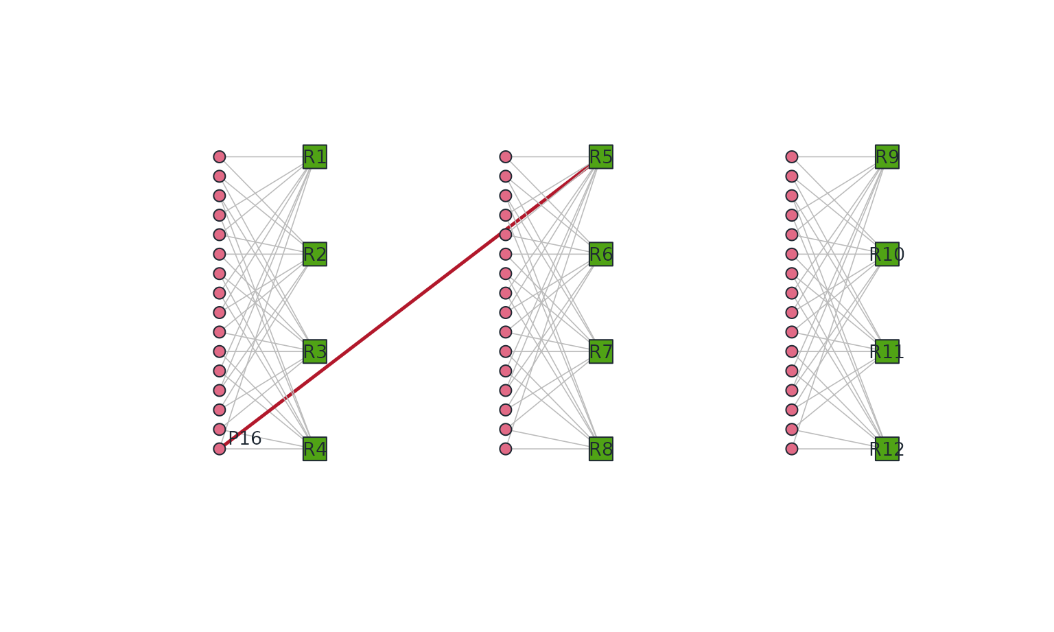
Planned person-rater assignments. Columns represent three panels; circles are persons and squares are raters. The red line links P16 to R5. The third panel remains disconnected; the added single link is fragile.

Adding a Criterion level shared by all rows would connect the graph through that node, even though person/rater locations in separate panels may still be confounded. Review both the person-rater projection and the full design; after fitting, inspect the model’s identification audit. A bridge is a vulnerability in the selected graph, not a test of the precision of a particular contrast. Degree counts neighbours; strength sums edge counts. Betweenness counts shortest paths and closeness uses inverse path distances. Here distances are inverse co-observation counts. Disconnected-node closeness is local to reachable nodes, so it should not rank raters across disconnected panels. Centrality is not accuracy, severity or importance to the construct.

Compare score networks with MFRM

Lamprianou (2025) illustrates exact agreement, signed agreement, directed score differences, rater-by-criterion correlations and comparisons with MFRM. Those views motivate the following richer example; the bundled synthetic data are not a replication of that study. Its strong NA–MFRM association is an empirical result, not an identity between a network index and a Rasch parameter. Lamprianou (2018) also investigates fitted exponential random graph models; these descriptive constructors do not fit those models.

if (requireNamespace("igraph", quietly = TRUE)) {
  fit <- fit_mfrm(ratings, "Person", c("Rater", "Criterion"), "Score",
    method = "JML", maxit = 300)
  diagnostics <- diagnose_mfrm(fit, residual_pca = "none")
  agreement <- rater_network_analysis(fit, diagnostics, mode = "agreement")
  directional <- rater_network_analysis(fit, diagnostics,
    mode = "severity_direction", score_diff_tolerance = 0, severity_continuity = .5)
}

In the directional graph an arrow goes from the higher-scoring rater to the lower-scoring rater on shared contexts. This is lenient-to-severe only when higher scores mean a more favourable performance. The index is -log((OutStrength + c)/(InStrength + c)); c = .5 is this package’s continuity choice, not the paper’s uncorrected formula. Missing overlap, tied scores and zero strengths must remain visible. Never interpret this index as calibrated logits or turn unavailable values into zero.

if (requireNamespace("igraph", quietly = TRUE)) {
  raters <- sort(directional$node_metrics$Rater)
  angle <- seq(0, 2*pi, length.out = length(raters) + 1L)[seq_along(raters)]
  coords <- cbind(cos(angle), sin(angle)); rownames(coords) <- raters
  old <- par(mfrow = c(1, 2), mar = c(1, 1, 1, 1))
  plot(agreement, type = "network", layout = coords,
    graphical = list(vertex.size = 13))
  sev <- directional$node_metrics$SeverityIndex
  sizes <- rep(10, length(sev)); ok <- is.finite(sev)
  if (any(ok)) sizes[ok] <- 10 + 8 * (sev[ok] - min(sev[ok])) / max(.01, diff(range(sev[ok])))
  plot(directional, type = "network", layout = coords,
    graphical = list(vertex.size = sizes, edge.curved = .2))
  par(old)
  comparison <- merge(directional$node_metrics[, c("Rater", "SeverityIndex")],
    subset(diagnostics$measures, Facet == "Rater", select = c(Level, Estimate, SE)),
    by.x = "Rater", by.y = "Level", all = TRUE)
  comparison
}

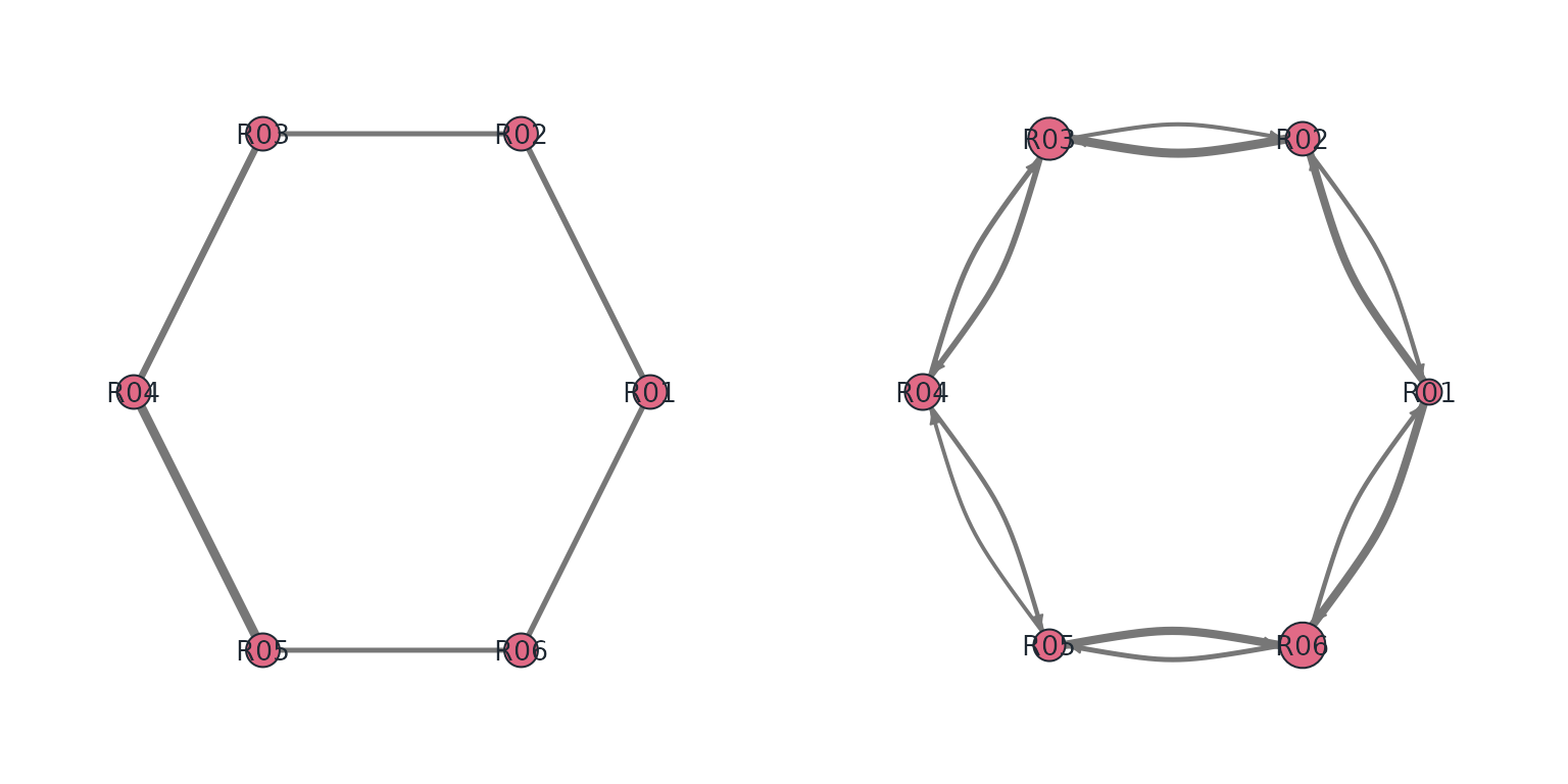
Observed agreement (left) and directional discrepancies (right), with the same rater positions. Edge widths represent the relevant proportions. In the right panel larger nodes have higher network severity indices, not greater statistical significance.

#>   Rater SeverityIndex    Estimate        SE
#> 1   R01   -0.38260697 -0.64335896 0.1945869
#> 2   R02   -0.08004271 -0.35687808 0.1797840
#> 3   R03    0.23515170  0.37432053 0.1954466
#> 4   R04    0.00000000  0.23506014 0.2034984
#> 5   R05   -0.14996859  0.03222081 0.2226887
#> 6   R06    0.36066697  0.35863557 0.2423906

Report the context keys, pair overlap, score-difference tolerance and weighting. min_weight in the constructor changes the calculated network. To reduce visual clutter without changing its statistics, use the plot argument display_min_weight. This follows the distinction between calculation and illustration in Lamprianou’s figures. Three further questions now connect to these same results:

if (requireNamespace("igraph", quietly = TRUE)) {
  signed <- rater_network_analysis(fit, diagnostics,
    weight_metric = "KrippendorffAlpha", alpha_level = "interval")
  signed$pair_metrics[, c("Rater1", "Rater2", "N", "KrippendorffAlpha", "AlphaStatus")]
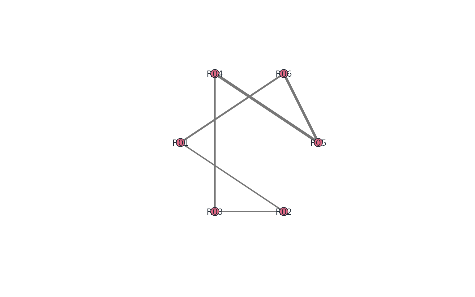
  plot(signed) # Negative agreement uses dashed edges; undefined pairs stay NA.
  magnitude <- rater_network_analysis(fit, diagnostics,
    mode = "severity_direction", weight_metric = "DirectionalMagnitude",
    severity_continuity = 0)
  magnitude$network_fit
}

Rater nodes joined by pairwise Krippendorff alpha edges. Width represents magnitude; negative edges, when present, are dashed. Unavailable pairs have no edge.

#>     Rater Partners Comparisons OutStrength InStrength SeverityIndex
#> R01   R01        2          46   1.1468254  0.5277778    -0.7760776
#> R02   R02        2          54   0.9807692  0.8049451    -0.1975632
#> R03   R03        2          49   0.7040134  1.0351171     0.3854724
#> R04   R04        2          46   0.5652174  0.6956522     0.2076394
#> R05   R05        2          43   0.7608696  0.5108696    -0.3983476
#> R06   R06        2          38   0.5277778  1.1111111     0.7444405
#>              SWS        PUS SWSStatus PUSStatus
#> R01  0.003744078 0.15184083 available available
#> R02 -0.184430101 0.16533707 available available
#> R03 -0.164246173 0.16453535 available available
#> R04 -0.302664967 0.10018904 available available
#> R05 -0.229340583 0.09652647 available available
#> R06  0.161693000 0.14737654 available available

Pairwise alpha adjusts agreement for the pair’s own score marginals. It is neither Pearson correlation nor the multi-rater alpha for the whole panel. Negative alpha remains negative. Zero agreement does not draw an edge; undefined agreement is unavailable, not zero. Ordinal alpha needs an explicit category order. SignedStrength distinguishes positive from negative ties; path centralities are withheld for signed alpha.

DirectionalMagnitude weights a comparison by the size of its score difference. The default directional network instead counts how often a rater scores higher. The network_fit table implements Lamprianou’s equations 1–3: raw network severity, SWS and PUS, calculated before graph filtering. SWS can be negative; undefined strength ratios stay unavailable. Multiplying all scores by a positive constant leaves severity unchanged but changes SWS and PUS. Report score units/range and never apply Rasch MnSq cutoffs to them. Use mfrm_report(magnitude) to retain the indices, definitions and caveats.

if (requireNamespace("igraph", quietly = TRUE)) {
  halo <- rater_halo_network_analysis(fit, diagnostics, method = "spearman",
    alpha = 1, min_pair_n = 5, positive_only = FALSE)
  nodes <- halo$node_metrics
  raters <- unique(nodes$Rater); criteria <- unique(nodes$Criterion)
  center <- 2*pi*(match(nodes$Rater, raters) - 1)/length(raters)
  corner <- 2*pi*(match(nodes$Criterion, criteria) - 1)/length(criteria)
  coords <- cbind(3*cos(center) + .65*cos(corner), 3*sin(center) + .65*sin(corner))
  rownames(coords) <- nodes$Node
  within_rater <- halo$edge_metrics$EdgeType == "halo"
  plot(halo, type = "network", layout = coords,
    graphical = list(vertex.label = paste(nodes$Rater, substr(nodes$Criterion, 1, 1), sep = "-"),
      vertex.size = 10, vertex.label.cex = .85,
      edge.color = ifelse(within_rater, "#2166AC", "#D4D4D4"),
      edge.width = .3 + 2.5 * abs(halo$edge_metrics$SignedWeight)))
  halo$halo_summary_by_rater
}

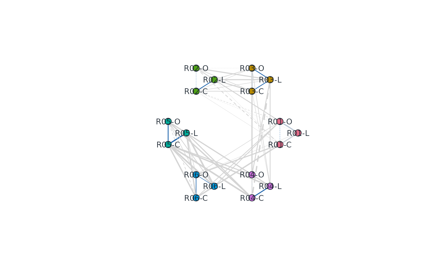
Rater-by-criterion observed-score network. Nodes are grouped by rater (C: Content, L: Language, O: Organization); blue lines join criteria scored by the same rater and grey lines join different raters. Width shows correlation magnitude; dashed lines indicate negative correlations. Correlation does not identify a causal halo effect.

#>   Rater ExpectedHaloPairs UnavailableHaloPairs ExpectedIncidentNonHaloPairs
#> 1   R03                 3                    0                           45
#> 2   R01                 3                    0                           45
#> 3   R05                 3                    0                           45
#> 4   R02                 3                    0                           45
#> 5   R06                 3                    0                           45
#> 6   R04                 3                    0                           45
#>   UnavailableIncidentNonHaloPairs UnavailableIncidentPValues HaloPairs
#> 1                              27                         27         3
#> 2                              27                         27         3
#> 3                              27                         27         3
#> 4                              27                         27         3
#> 5                              27                         27         3
#> 6                              27                         27         3
#>   RetainedHaloEdges RetainedHaloShare MeanHaloWeight MeanRetainedHaloWeight
#> 1                 3                 1      0.4464282              0.4464282
#> 2                 3                 1      0.3003553              0.3003553
#> 3                 3                 1      0.5122876              0.5122876
#> 4                 3                 1      0.1556369              0.1556369
#> 5                 3                 1      0.3287357              0.3287357
#> 6                 3                 1      0.2838713              0.2838713
#>   MaxHaloWeight MeanSignedHaloWeight IncidentNonHaloPairs
#> 1     0.5897645            0.4464282                   18
#> 2     0.4564516            0.2724915                   18
#> 3     0.7113284            0.5122876                   18
#> 4     0.4004971            0.1457486                   18
#> 5     0.5121024            0.3287357                   18
#> 6     0.5196888            0.2838713                   18
#>   MeanIncidentNonHaloWeight HaloMinusIncidentNonHalo HaloRatioIncident
#> 1                 0.3867314               0.05969686         1.1543626
#> 2                 0.2683811               0.03197415         1.1191371
#> 3                 0.5865107              -0.07422303         0.8734498
#> 4                 0.2624900              -0.10685309         0.5929251
#> 5                 0.4483916              -0.11965591         0.7331442
#> 6                 0.5307416              -0.24687028         0.5348578
#>   ReviewStatus
#> 1       review
#> 2       review
#> 3       review
#> 4       review
#> 5       review
#> 6       review
#>                                                                                                                                                                                                                                                                                                           ReviewReason
#> 1  Mean halo weight 0.446; incident non-halo mean 0.387; halo contrast 0.060; retained halo edges 3/3. The same-rater or other-rater comparison is incomplete; absence of a flag is not evidence against halo. 27 incident pair p-value(s) are unavailable. The p filter was disabled; retained edges are descriptive.
#> 2  Mean halo weight 0.300; incident non-halo mean 0.268; halo contrast 0.032; retained halo edges 3/3. The same-rater or other-rater comparison is incomplete; absence of a flag is not evidence against halo. 27 incident pair p-value(s) are unavailable. The p filter was disabled; retained edges are descriptive.
#> 3 Mean halo weight 0.512; incident non-halo mean 0.587; halo contrast -0.074; retained halo edges 3/3. The same-rater or other-rater comparison is incomplete; absence of a flag is not evidence against halo. 27 incident pair p-value(s) are unavailable. The p filter was disabled; retained edges are descriptive.
#> 4 Mean halo weight 0.156; incident non-halo mean 0.262; halo contrast -0.107; retained halo edges 3/3. The same-rater or other-rater comparison is incomplete; absence of a flag is not evidence against halo. 27 incident pair p-value(s) are unavailable. The p filter was disabled; retained edges are descriptive.
#> 5 Mean halo weight 0.329; incident non-halo mean 0.448; halo contrast -0.120; retained halo edges 3/3. The same-rater or other-rater comparison is incomplete; absence of a flag is not evidence against halo. 27 incident pair p-value(s) are unavailable. The p filter was disabled; retained edges are descriptive.
#> 6 Mean halo weight 0.284; incident non-halo mean 0.531; halo contrast -0.247; retained halo edges 3/3. The same-rater or other-rater comparison is incomplete; absence of a flag is not evidence against halo. 27 incident pair p-value(s) are unavailable. The p filter was disabled; retained edges are descriptive.

alpha = 1 here avoids a significance filter; counts and unavailable pairs are still reviewed. Same-rater correlations can reflect real trait covariance, range restriction and rubric overlap. The package preserves descriptive within-/between-rater comparisons. For uncertainty, resample persons, keeping all their criteria, raters and repeated contexts together:

halo_ci <- rater_halo_network_analysis(fit, diagnostics, alpha = 1,
  positive_only = FALSE, bootstrap = 999, seed = 47,
  halo_reference = "different_criteria")
halo_ci$halo_contrast
halo_ci$bootstrap_draws # All attempts, including undefined fixed-pair draws.
mfrm_report(halo_ci)

The contrast averages signed within-rater cross-criterion correlations and subtracts the between-rater cross-criterion mean. halo_reference = "all" includes same-criterion reference edges, as in the paper’s descriptive comparison. These are different targets. Check the criterion-pair mix and shared-person counts in contrast_pairs; neither automatically balances a sparse design. The contrast uses unfiltered correlations, so display or significance filtering does not select its target.

Intervals are approximate and conditional on the observed raters/criteria and pair set. They require independent, representative person clusters and enough variation. This sparse example can produce undefined bootstrap correlations; the returned status is then incomplete_bootstrap, with an unavailable interval and the failure denominator retained. Increasing resamples does not repair poor overlap. Inspect the design and report the limitation. An independent-edge Welch test is not an alternative: edges share raters and persons. Residual networks instead ask what remains after the fitted model and are documented in ?mfrm_residual_network; they cannot automatically establish causal halo either.

Model network configurations with ERGM

Use ERGM when the research question concerns the network: for example, whether leniency ties are reciprocated, or whether a supplied rater attribute is associated with ties after accounting for network structure. This does not replace the MFRM or convert its severity into a network coefficient.

# An explicit tie definition: pairwise interval alpha > 0.35.
# Missing pairs are modeled only under an ignorable missingness assumption.
model <- fit_rater_network(signed, ~ edges, threshold = 0.35,
  missing = "model", seed = 48, gof = ~ degree,
  gof_control = ergm::control.gof.ergm(nsim = 199, seed = 49))
model$dyads # NA is unobserved; 0 is an observed non-tie.
model$coefficients
model$diagnostics
plot(model, type = "gof")
report <- mfrm_report(model)
export_summary_appendix(report, output_dir = "network-report", prefix = "ergm")

The six-rater example is a demonstration of data handoff, not evidence that a complex ERGM is estimable. For a substantively supported directed network, ~ edges + mutual asks about reciprocal ties; exogenous node covariates can be supplied as node_data with a unique Node column, then referenced by terms such as nodecov("Experience"). More complex terms can require MCMC: inspect ergm::mcmc.diagnostics(model$fit) for mixing and effective sample size, then simulated GOF. A returned object is not an automatic convergence certificate. The original backend object is retained for further diagnostics.

Both edges and non-edges must be observed. No overlap or an undefined alpha is not a non-edge. By default the wrapper refuses such data; the explicit missing = "model" option assumes ignorable missingness, which may be implausible for informative assignment or constant scores. Binarization uses all eligible pair values before graph filtering. Report its metric, cutoff, strict inequality, overlap rule and missingness assumption. Compare plausible thresholds as sensitivity analyses, not by minimizing AIC across different response networks. The wrapper does not fit valued/signed ERGMs or propagate uncertainty in estimated pairwise edges.

All three network routes now connect to mfrm_report() and export_summary_appendix(). They preserve full pair/dyad tables, unavailable states and calculation settings. For custom figures use plot_data(plot(x, draw = FALSE)), x$bootstrap_draws, or x$gof_draws; draws are in long form. Your methods and results still need the substantive question, rater sampling, rubric direction, missingness, the declared network definition and a reasoned interpretation. A large contrast alone is not evidence of causal halo.

Connect to a manuscript, not a coefficient inventory

Use the reporting guide to choose modules by question. The following primary-source examples explain why those modules belong together. They are examples of reporting practice, not universal rules.

Source examined	Reported evidence	Connection and qualification
FACETS Table 7 and reliability help	Facet measures/errors, fit, separation/strata/reliability, and separate agreement statistics	`diagnose_mfrm()` → `mfrm_results()` → `mfrm_report()`; declare Model/Real and sample/population conventions. Rater separation reliability concerns distinguishable severities, not agreement.
ConQuest `show` and technical manual	Parameter estimates/errors/fit, population distributions/reliability, maps, thresholds, and model-comparison information	Use fitted-model summaries, category curves and `compare_mfrm()` together. ConQuest MML fit definitions are not the package’s EAP plug-in summaries; match model, score coding, constraints and estimator before numerical comparison.
Koizumi et al. (2019), speaking, Tables 4–9 and Wright map	Facet means/SD/SE, separation/strata/reliability; fit, agreement and categories; task variance and absolute-decision D-studies	Their MFRM used three facets; their G-study used person × task, with single/averaged rater scores. This is a declared change of unit and target, not an automatic conversion of a fitted object.
Lin Chun & Xiao Yunnan (2018), EFL writing, Tables I–VI	Variance components/SE/percentages; G across rater counts; rater severity/fit and rater-by-dimension/person bias	Combine planning with specified bias questions. This conference study used a score-stratified sample and one writing topic. Its sufficient-rater count and unadjusted bias thresholds do not generalize to other rubrics, populations or multiplicity policies.

The two studies used different scoring designs. In a combined manuscript, record separately for MFRM and G/D: input rows and retained persons, the observed or latent target, facets, aggregation, weights, sampling universe, and direction. Explain why each analysis answers a different part of the assessment question. For example: MFRM locates specific severity/misfit patterns; a G-study partitions variation in an explicitly defined observed score; a D-study projects its error under specified future counts. G/Phi are not additional independent validations of a Rasch reliability coefficient. Rasch-adjusted person estimates do not become raw G-study observations merely by putting them in a column named Score.

Copy templates/gpcm-report.Rmd and/or templates/gtheory-report.Rmd from system.file("templates", package = "mfrmr"). Their tables are editable, not mandatory journal layouts. The GPCM report includes optional paired-kappa code. For linking, retain the anchor source/scale, fixed-versus-estimated status and drift review. For bias, report signed effects, cell support, multiplicity and uncertainty, not just a list of flagged raters. For model comparison, retain the comparable-data/likelihood decision, changes in substantive estimates and unavailable tests. Those modules are linked from the reporting guide; the GPCM example does not claim to execute every one of them.

Export values and choose your own graphics

plot_data(picture, "nodes"), plot_data(picture, "edges") and plot_data(picture, "coordinates") provide editable graph data. source_edges keeps the calculated graph when the picture is filtered. Graph views do not automatically convert with as_ggplot(); use these tables with your chosen graph library. For matrices, use plot_data(p, "matrix", format = "long"); for a wide table, select explicit value_cols with format = "long". Missing cells and identifiers remain. A long table does not make unlike quantities comparable.

write.csv(plot_data(picture, "nodes"), "design-nodes.csv", row.names = FALSE)
write.csv(plot_data(picture, "source_edges"), "design-edges.csv", row.names = FALSE)
saveRDS(list(network = after, plot = picture), "design-review.rds")
# For a fitted clustering result:
raw <- plot_data(groups, "observations", type = "profile", feature = "ExperienceYears")
write.csv(raw, "feature-observations.csv", row.names = FALSE)

The feature lesson shows an editable raincloud plot from the new observations component. It retains individual values, cluster membership, missingness and inclusion. Parameter summaries, SEs and interval bounds are not raw replicates or posterior draws. Do not draw their density as if they were. Raw repeated rating rows are also not independent persons. Keep analysis objects as RDS alongside CSVs to retain types, settings and interpretation notes.

References

Lamprianou, I. (2025). Network analysis for the investigation of rater effects in language assessment: A comparison of ChatGPT vs human raters. Research Methods in Applied Linguistics, 4, 100205. https://doi.org/10.1016/j.rmal.2025.100205.
Lamprianou, I. (2018). Investigation of rater effects using social network analysis and exponential random graph models. Educational and Psychological Measurement, 78, 430–459. https://doi.org/10.1177/0013164416689696.
Koizumi, R., Kaneko, E., Setoguchi, E., In’nami, Y., & Naganuma, N. (2019). Examination of CEFR-J spoken interaction tasks using many-facet Rasch measurement and generalizability theory. Papers in Language Testing and Assessment, 8(2), 1–33. https://doi.org/10.58379/BSWY7332.
Lin Chun & Xiao Yunnan (2018). A study on rater reliability under holistic and analytic scoring of CEPT writing by using generalizability theory and many-facet Rasch model. Proceedings of EMLE 2018, 1013–1019. https://doi.org/10.2991/emle-18.2018.201.
FACETS: Table 7 and reliability, separation and strata.
ACER ConQuest: output commands and technical description.